Singular Value Decomposition (SVD)

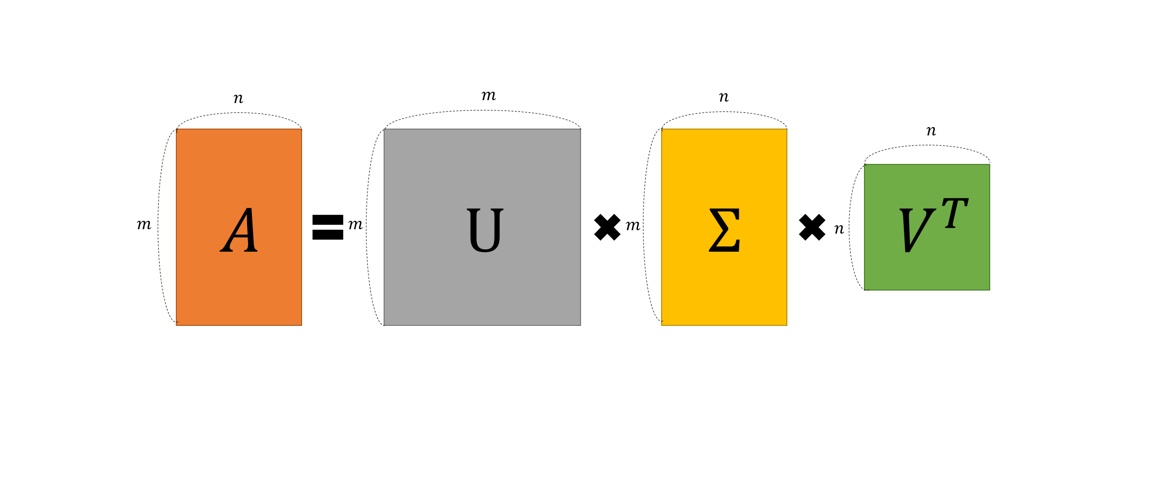
Singular Value Decomposition (SVD) is a mathematical technique that factorizes a matrix $A$ into three simpler matrices: $U$, $Σ$, and $V^T$. This decomposition allows us to express the original matrix as a product of these matrices, which makes it easier to analyze and manipulate.The formula for SVD is:

\[A = U Σ V^T\]

Where:

• $A$ is an $m×n$ matrix,
• $U$ is an $m×m$ orthogonal matrix (left singular vectors),
• $Σ$ is an $m×n$ diagonal matrix (singular values),
• $V^T$ is the transpose of an $n×n$ orthogonal matrix (right singular vectors).

This decomposition has a range of applications in unsupervised learning (like PCA), recommendation systems (like Netflix and Amazon), and Google’s PageRank algorithm.

Components of SVD

• Matrix $U$ (Left Singular Vectors) : $U$ contains the left singular vectors of matrix $A$. These vectors are orthogonal,meaning all of its columns are linearly independent, and describe the directions in the original space that are most important. These are the eigenvectors of $AA^T$.
• Matrix $Σ$ (Singular Values): The diagonal matrix $Σ$ contains the singular values, which represent the importance or strength of each component. The singular values are the square roots of the eigenvalues of $A^TA$ (or $AA^T$) and are always non-negative. This tells us how important each direction is.
• Matrix $V$ contains the right singular vectors of $A$, and when transposed (as $V^T$), it tells us how the data points are distributed in the feature space. These are the eigenvectors of $A^TA$.

Each of these matrices($U,\Sigma,V$) helps us understand the original matrix in a deeper way. It’s like taking apart a machine to see how all the parts work together!

Mathematical Foundation of SVD

SVD is closely related to eigenvalue decomposition, which you may have encountered before. To understand this, let’s recall that the eigenvectors and eigenvalues of a matrix $A$ are solutions to the equation:

\[Av=λv\]

Where $v$ is an eigenvector and $λ$ is its corresponding eigenvalue. SVD builds on this by decomposing $A$ into three matrices based on eigenvalues and eigenvectors of $A^TA$ and $AA^T$.

Eigenvalue Decomposition and SVD:

• Eigenvectors of $AA^T$ form the columns of $U$.
• Eigenvectors of $A^TA$ form the columns of $V$.
• The square roots of eigenvalues of $A^TA$ (or $AA^T$) form the singular values in $Σ$.

---

Eigenvalues and Eigenvectors: What Are They?

It may be true

To understand SVD, we need to know about eigenvalues and eigenvectors. These are concepts from linear algebra that help us understand transformations (how things like matrices can stretch or rotate a shape).

• Eigenvectors are special vectors that don’t change direction when a matrix is applied to them. They can stretch or shrink but always point in the same direction.

• Eigenvalues tell us how much the eigenvectors stretch or shrink. A large eigenvalue means the vector stretches a lot, while a small eigenvalue means it shrinks.

Imagine pushing on a piece of elastic. The eigenvector is the direction in which the elastic stretches, and the eigenvalue is how far it stretches.

In SVD, the eigenvalues are connected to the singular values, and the eigenvectors make up the U and V matrices. Together, they give us a way to understand the directions in which the matrix “pulls” the data. If you want to learn more about eigen vectors and eigen values, i highly recommended you to watch 3Blue1Brown’s video

Image Source Wikimedia

Subspaces and Dimensions: What Are We Doing with the Data?

In simple terms, SVD helps us break down a complex dataset into smaller, simpler parts that are easier to work with.

• Subspaces: A subspace is like a lower-dimensional version of a space. If we have a bunch of data points in 3D space (like the x, y, z coordinates), we can use SVD to project those points onto a 2D plane (like x, y coordinates), which makes the data easier to work with.

• Dimensionality Reduction: Sometimes, we have too many dimensions (features) in our data, and that makes things complicated. SVD allows us to reduce the number of dimensions while keeping the most important information. This is called dimensionality reduction.

How Does SVD Help in Machine Learning?

SVD is often used in unsupervised learning techniques for machine learning. One of its main uses is to reduce the dimensionality of a dataset. Why is Dimensionality Reduction Important?

In high-dimensional datasets (like images, text, or big datasets with lots of features), a lot of the information might be redundant or unimportant. Reducing the number of dimensions can:

• Speed up computation.
• Make models easier to interpret.
• Prevent the curse of dimensionality, which can cause models to overfit.

By keeping only the most important singular values, we can reduce the number of features in the dataset while still keeping the most important information.

Applications of SVD in Real-World Problems

• Recommendation Systems (Netflix, Amazon):
  When you watch a movie or buy something online, companies like Netflix and Amazon use SVD to analyze your preferences and recommend other movies or products. They decompose a user-item interaction matrix using SVD and predict what you might like based on similar patterns.

• Google PageRank:
  Google uses SVD in its PageRank algorithm, which helps rank web pages by their importance. It analyzes how web pages are linked and uses SVD to find patterns in those links.

• Image Compression:
  SVD can also be used to compress images. By decomposing the image into singular values and truncating the less important ones, we can reduce the file size without losing much visual quality.

Projection of Principal Component1.gif

SVD in Matrix Form

Given a matrix $A$, the SVD is:

\[A = U \Sigma V^T\]

Where $U$, $Σ$, and $V^T$ look like:

\[\rightarrow U = [u_1​,u_2​,...,u_m​ ]_{1xm} \ \text{(left singular vectors)}\] \[\rightarrow \ \Sigma = diag(σ_1,σ_2,...,σ_k) \ \text{(singular values)}\] \[\rightarrow \ V^T = \begin{bmatrix} v_1^T \\ v_2^T \\ \vdots \\ v_n^T \end{bmatrix} \text{(right singular vectors)}\]

Key Properties:

• $U$ and $V$ are orthogonal matrices, meaning their columns are unit vectors and $U^TU=I$ and $V^TV=I$
• $Σ$ contains non-negative singular values $σ_1≥σ_2≥…≥σ_k≥0$

An Example of SVD with Detailed Calculations

Let’s work through a simple numerical example to demonstrate how to calculate the SVD of a matrix. Consider a matrix:

\[A = \begin{bmatrix} 1 & 2 \\ 3 & 3 \end{bmatrix}\]

Step 1: Compute $A^TA$ and $AA^T$

\[A A^T = \begin{bmatrix} 1 & 2 \\ 3 & 3 \end{bmatrix} \begin{bmatrix} 1 & 3 \\ 2 & 3 \end{bmatrix} = \begin{bmatrix} 5 & 9 \\ 9 & 18 \end{bmatrix}\] \[A^T A = \begin{bmatrix} 1 & 3 \\ 2 & 3 \end{bmatrix} \begin{bmatrix} 1 & 2 \\ 3 & 3 \end{bmatrix} = \begin{bmatrix} 10 & 11 \\ 11 & 13 \end{bmatrix}\]

Step 2: Compute Eigenvalues

\[\text{det}(A A^T - \lambda I) = 0\] \[A A^T = \begin{bmatrix} 1 & 2 \\ 3 & 3 \end{bmatrix} \begin{bmatrix} 1 & 3 \\ 2 & 3 \end{bmatrix} = \begin{bmatrix} 5 & 9 \\ 9 & 18 \end{bmatrix} - \begin{bmatrix} \lambda & 0 \\ 0 & \lambda \end{bmatrix}\] \[\text{det} \begin{bmatrix} 5 - \lambda & 9 \\ 9 & 18 - \lambda \end{bmatrix} = (5 - \lambda)(18 - \lambda) - 81 = 0\] \[(5 - \lambda)(18 - \lambda) - 81 = \lambda^2 - 23\lambda + 9 = 0\]

$ \text(roots \ of \ an \ equation) = \Large \frac{-b \pm \sqrt{b^2 - 4ac}}{2a} $

\[\lambda = \frac{23 \pm \sqrt{23^2 - 4 \cdot 1 \cdot 9}}{2 \cdot 1} = \frac{23 \pm \sqrt{493}}{2}\] \[\lambda_1 = \frac{23 + \sqrt{493}}{2} \approx 22.6\] \[\lambda_2 = \frac{23 - \sqrt{493}}{2} \approx 0.4\]

Step 3: Calculate Singular Values

The singular values are the square roots of the eigenvalues

$ \sigma_1 = \sqrt \lambda_1 = \sqrt 22.6 \approx 4.76 \\ \ \sigma_2 = \sqrt \lambda_2 = \sqrt 0.4 \approx 0.63 $

\[\Sigma = \begin{bmatrix} 4.76 & 0 \\ 0 & 0.63 \end{bmatrix}\]

Step 4: Compute Eigenvectors of $AA^T$ ($U$)

Let’s calculate eigenvector for first eigen value $λ_1 = 22.6:$

\[A A^T - \lambda_1 I = \begin{bmatrix} 5 - 22.6 & 9 \\ 9 & 18 - 22.6 \end{bmatrix} = \begin{bmatrix} -17.6 & 9 \\ 9 & -4.6 \end{bmatrix}\] \[\begin{bmatrix} -17.6 & 9 \\ 9 & -4.6 \end{bmatrix} \begin{bmatrix} u_1 \\ u_2 \end{bmatrix} = \begin{bmatrix} 0 \\ 0 \end{bmatrix}\] \[-17.6\cdot u_1 + 9\cdot u_2 = 0\] \[u_2 = \frac{17.6}{9} \times u_1 \approx 1.96 \times u_1\] \[\| u \| = \sqrt{u_1^2 + u_2^2} = \sqrt{u_1^2 + (1.96 \cdot u_1)^2} = u_1 \sqrt{1 + 1.96^2} = u_1 \times \sqrt{4.82}\] \[u_1 = \frac{1}{\sqrt{4.82}} \approx 0.46\] \[u_2 = 1.96 \times 0.46 \approx 0.89\] \[U_1 = \begin{bmatrix} 0.46 \\ 0.89 \end{bmatrix}\]

Calculate other eigen vector for eigen value $\lambda_2=0.4$:

\[A A^T - \lambda_2 I = \begin{bmatrix} 5 - 0.4 & 9 \\ 9 & 18 - 0.4 \end{bmatrix} = \begin{bmatrix} 4.6 & 9 \\ 9 & 17.6 \end{bmatrix}\] \[\begin{bmatrix} 4.6 & 9 \\ 9 & 17.6 \end{bmatrix} \begin{bmatrix} u_1 \\ u_2 \end{bmatrix} = \begin{bmatrix} 0 \\ 0 \end{bmatrix}\] \[4.6 \cdot u_1 + 9 \cdot u_2 = 0\] \[u_2 = -\frac{4.6}{9} u_1 \approx -0.51 \times u_1\] \[\| u \| = \sqrt{u_1^2 + u_2^2} = \sqrt{u_1^2 + (-0.51 u_1)^2} = u_1 \sqrt{1 + 0.26} = u_1 \times \sqrt{1.26}\] \[u_1 = \frac{1}{\sqrt{1.26}} \approx 0.89\] \[u_2 = -0.51 \times 0.89 \approx -0.45\] \[U_2 = \begin{bmatrix} 0.89 \\ -0.45 \end{bmatrix}\]

\[U = \begin{bmatrix} 0.46 & 0.89 \\ 0.89 & -0.45 \end{bmatrix} \ \text(Left\ Singular\ Values)\]

Step 5: Compute Eigenvectors of $A^TA$ ($V$)

Eigenvalues are same for both $U$ and $V$ matrices, we already have calculated eigenvalues for $U$ matrix. So there is no need to re-calculate again. However, for proving that their eigen values are same, lets re-calculate only determinant of $A^TA$.

\[\text Question :: det(A^TA-\lambda I) = det(AA^T-\lambda I) = \lambda^2 - 23\lambda + 9\] \[A^T A - \lambda I= \begin{bmatrix} 1 & 3 \\ 2 & 3 \end{bmatrix} \begin{bmatrix} 1 & 2 \\ 3 & 3 \end{bmatrix} - \lambda I = \begin{bmatrix} 10 & 11 \\ 11 & 13 \end{bmatrix} - \begin{bmatrix} \lambda & 0 \\ 0 & \lambda \end{bmatrix}\] \[\text{det} \begin{bmatrix} 10 - \lambda & 11 \\ 11 & 13 - \lambda \end{bmatrix} = (10 - \lambda)(13 - \lambda) - 121 =0\] \[(5 - \lambda)(18 - \lambda) - 121 = \lambda^2 - 23\lambda + 9 = 0\]

As you can see above, both determinant are same. So there is no need to re-calculate eigenvalues again. We know that eigen value $\lambda_1$ = 22.6 and $\lambda_2$ = 0.4

Let’s calculate eigenvector for first eigen value $λ_1 = 22.6:$

\[A A^T - \lambda_1 I = \begin{bmatrix} 10 - 22.6 & 11 \\ 11 & 13 - 22.6 \end{bmatrix} = \begin{bmatrix} -12.6 & 11 \\ 11 & -9.6 \end{bmatrix}\] \[\begin{bmatrix} -12.6 & 11 \\ 11 & -9.6 \end{bmatrix} \begin{bmatrix} v_1 \\ v_2 \end{bmatrix} = \begin{bmatrix} 0 \\ 0 \end{bmatrix}\] \[-12.6\cdot v_1 + 11\cdot v_2 = 0\] \[v_2 = \frac{12.6}{11} \times v_1 \approx 1.45 \times v_1\] \[\| v \| = \sqrt{v_1^2 + v_2^2} = \sqrt{v_1^2 + (1.45 \cdot v_1)^2} = v_1 \sqrt{1 + 1.45^2} = v_1 \times \sqrt{2.31}\] \[v_1 = \frac{1}{\sqrt{2.31}} \approx 0.65\] \[v_2 = 1.45 \times 0.65 \approx 0.95\] \[V_1 = \begin{bmatrix} 0.65 \\ 0.95 \end{bmatrix}\]

Calculate other eigen vector for eigen value $\lambda_2=0.4$:

\[A A^T - \lambda_2 I = \begin{bmatrix} 10 - 0.4 & 11 \\ 11 & 13 - 0.4 \end{bmatrix} = \begin{bmatrix} 9.6 & 11 \\ 11 & 12.6 \end{bmatrix}\] \[\begin{bmatrix} 9.6 & 11 \\ 11 & 12.6 \end{bmatrix} \begin{bmatrix} v_1 \\ v_2 \end{bmatrix} = \begin{bmatrix} 0 \\ 0 \end{bmatrix}\] \[9.6 \cdot v_1 + 11 \cdot v_2 = 0\] \[v_2 = -\frac{9.6}{11} v_1 \approx -0.87 \times v_1\] \[\| v \| = \sqrt{v_1^2 + v_2^2} = \sqrt{v_1^2 + (-0.87 v_1)^2} = v_1 \sqrt{1 + 0.76} = v_1 \times \sqrt{1.76}\] \[v_1 = \frac{1}{\sqrt{1.76}} \approx 1.32\] \[v_2 = -0.87 \times 1.32 \approx -1.15\] \[V_2 = \begin{bmatrix} 1.32 \\ -1.15 \end{bmatrix}\]

\[V = \begin{bmatrix} 0.65 & 1.32 \\ 0.95 & -1.45 \end{bmatrix} \ \text(Right\ Singular\ Values)\]

Step 6: Verification

Now, we applied singular value decomposition method for $A$ matrix.

\[U = \begin{bmatrix} 0.65 & 1.32 \\ 0.95 & -1.45 \end{bmatrix}, \quad \Sigma = \begin{bmatrix} 4.76 & 0 \\ 0 & 0.63 \end{bmatrix} , \quad V = \begin{bmatrix} 0.8 & -0.6 \\ 0.6 & 0.8 \end{bmatrix}\]

Thus, the SVD decomposition is :

\[A = U \Sigma V^T = \begin{bmatrix} 0.65 & 1.32 \\ 0.95 & -1.45 \end{bmatrix} \cdot \begin{bmatrix} 4.76 & 0 \\ 0 & 0.63 \end{bmatrix} \cdot \begin{bmatrix} 0.8 & -0.6 \\ 0.6 & 0.8 \end{bmatrix}^T\]

Truncated to $r$ - Rank

Let’s say we want to truncate or dimension reduction to rank 1 for A matrix. We can do this step by step:

• Step 1: Analyze the Singular Value Matrix $\Sigma$
• Step 2: Truncate the Left Singular Matrix $U$
• Step 3: Truncate the Right Singular Matrix $V^T$
• Step 4: Reconstruct the Rank-1 Truncated Matrix $A_1$

Step 1: Analyze the Singular Value Matrix $\Sigma$

The diagonal matrix $\Sigma$ contains the singular values, which are non-negative and arranged in descending order. In this case, the matrix $\Sigma$ is:

\[\begin{bmatrix} 4.76 & 0 \\ 0 & 0.63 \end{bmatrix}\]

For rank-1 truncation, we only keep the largest singular value, which is $4.76$. We discard the smaller singular value $0.63$.

Thus, the truncated $\Sigma_1$ matrix become:

\[\Sigma_1 = \begin{bmatrix} 4.76 & 0 \end{bmatrix} \rightarrow first (i,j) \rightarrow (1,1)\]

Step 2: Truncate the Left Singular Matrix $U$

The matrix $U$ contains the left singular vectors. It is:

\[\begin{bmatrix} 0.65 & 1.32 \\ 0.95 & -1.45 \end{bmatrix}\]

Each column in $U$ corresponds to a singular value in $\Sigma$. Since we are doing a rank-1 truncation and only keeping the largest singular value, we need to keep only the first column of $U$, which corresponds to the largest singular value $4.76$. Thus, the truncated $U_1$ matrix becomes:

\[U_1 = \begin{bmatrix} 0.65 \\ 0.95 \end{bmatrix}\]

Step 3: Truncate the Right Singular Matrix $V^T$

The matrix $V^T$ contains the right singular vectors and is the transpose of $V$. It is:

\[V = \begin{bmatrix} 0.8 & -0.6 \\ 0.6 & 0.8 \end{bmatrix} \rightarrow V^T = \begin{bmatrix} 0.8 & 0.6 \\ -0.6 & 0.8 \end{bmatrix}\]

Similar to $U$, each row of $V^T$ corresponds to a singular value in $\Sigma$. For rank-1 truncation, we keep only the first row of $V^T$, which corresponds to the largest singular value $4.76$.

Thus, the truncated $V_1^T$ matrix becomes:

\[V_1^T = \begin{bmatrix} 0.8 & 0.6 \end{bmatrix}\]

Step 4: Reconstruct the Rank-1 Truncated Matrix $A_1$

Now, we can multiply the truncated matrices $U_1$, $\Sigma_1$​, and $V_1^T$​ to get the rank-1 approximation $A_1$

The formula for this multiplication is:

\[A_1 = U_1 \cdot \Sigma_1 ​\cdot V_1^T\]

Let’s calculate this step by step.

Multiply $U_1$​ and $\Sigma_1$ :

\[\begin{bmatrix} 0.65 \\ 0.95 \end{bmatrix}_{2\times1} \begin{bmatrix} 4.76 \end{bmatrix}_{1\times1} = \begin{bmatrix} 0.65 \times 4.76 \\ 0.95 \times 4.76 \end{bmatrix}_{2\times1} = \begin{bmatrix} 3.09 \\ 4.52 \end{bmatrix}_{2\times1}\]

Let’s multiply $V_1^T$ with result ,so $(U_1 \cdot \Sigma_1) \cdot V_1^T $

\[\begin{bmatrix} 3.09 \\ 4.52 \end{bmatrix}_{2\times1} \cdot \begin{bmatrix} 0.8 & 0.6 \end{bmatrix}_{1\times2} = \begin{bmatrix} 3.09 \times 0.8 & 3.09 \times 0.6 \\ 4.52 \times 0.8 & 4.52 \times 0.6 \end{bmatrix}_{2\times2} = \begin{bmatrix} 2.47 & 1.85 \\ 3.62 & 2.71 \end{bmatrix}_{2\times2}\]

The rank-1 truncated matrix $A_1$​ is:

\[A_1 = \begin{bmatrix} 2.47 & 1.85 \\ 3.62 & 2.71 \end{bmatrix}_{2\times2}\]

---

Step-by-Step SVD in Python

• Install NumPy to work with matrices : pip install numpy
• Perform SVD with NumPy

import numpy as np

# Create a simple matrix
A = np.array([[1, 2],
              [3, 3]])

# Perform Singular Value Decomposition
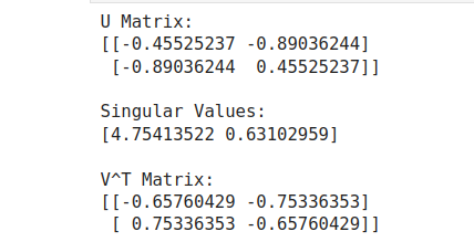
U, S, VT = np.linalg.svd(A)

print("U Matrix:")
print(U)

print("\nSingular Values:")
print(S)

print("\nV^T Matrix:")
print(VT)

• Reconstruct Matrix

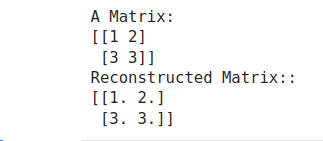
# Reconstruct the original matrix
S_diag = np.diag(S)
A_reconstructed = U @ S_diag @ VT

print("\nReconstructed Matrix:")
print(A_reconstructed)

• Truncated SVD (for rank-1)

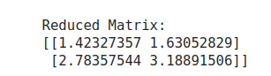
# Truncate to 1 dimensions
k = 1
U_k = U[:, :k]
S_k = np.diag(S[:k])
VT_k = VT[:k, :]

# Reconstruct with reduced dimensions
A_reduced = U_k @ S_k @ VT_k

print("\nReduced Matrix:")
print(A_reduced)

Last but not least, you can use Singular Value Decomposition with scikit-learn Truncated_SVD.

Conclusion

Singular Value Decomposition is a powerful tool in the data scientist’s toolbox, enabling dimensionality reduction, latent feature extraction, and matrix approximation. Its applications range from recommendation systems to graph algorithms and data compression. Understanding the underlying mathematics and how to implement SVD in Python allows you to harness the full power of this technique in machine learning and data science workflows.

By leveraging SVD, you can reduce computational complexity and make your models more efficient, interpretable, and faster!