Naive Bayes Simplified | From Theory to Code
Naive Bayes is a family of probabilistic classifiers based on Bayes' theorem with the "naive" assumption that features are conditionally independent given the class label. Despite this simplification, Naive Bayes classifiers often perform remarkably well on a variety of problems, especially with text classification and real-world datasets. This blog post explores the foundation of Bayes' theorem, its formula, and applications in real life.

Introduction
In the realm of machine learning and statistical classification, Naive Bayes stands out as one of the simplest and most effective algorithms. Its name stems from the “naive” assumption of feature independence, which, despite being a strong assumption, often leads to surprisingly accurate results. This blog post will guide you through the fundamental concepts of Naive Bayes, demonstrating its utility through real-life examples and a detailed step-by-step mathematical exploration. We will also cover various types of Naive Bayes classifiers, each tailored for different types of data, and implement them from scratch in Python.
Bayes’ Theorem: Foundation and Formula
Bayes’ theorem is a fundamental concept in probability theory and statistics, providing a way to update the probability of a hypothesis based on new evidence. It is named after the Reverend Thomas Bayes, who formulated it in the 18th century.
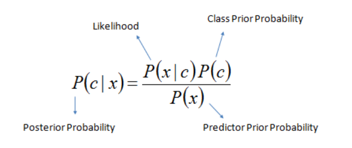
The formula for Bayes’ theorem is:
\[P(C \mid x) = \frac{P(x \mid C) \cdot P(C)}{P(x)}\]Where:
- $P(C∣x)$ is the posterior probability of class $C$ given the feature $x$.
- $P(x∣C)$ is the likelihood of feature $x$ given class $C$.
- $P(C)$ is the prior probability of class $C$.
- $P(x)$ is the marginal probability of feature $x$.
Foundation: Bayes’ theorem provides a way to update our beliefs about the likelihood of a class given new evidence. In classification problems, this means we can calculate the probability of a data point belonging to a particular class based on its features.
Real-Life Usage Examples
Spam Filtering: Naive Bayes is widely used in email spam filters. By analyzing the frequency of words in spam and non-spam emails, the classifier can predict whether a new email is spam.
Text Classification: In sentiment analysis or document categorization, Naive Bayes can classify text into different categories based on the frequency of words.
Medical Diagnosis: Naive Bayes can be used to predict the likelihood of a disease based on symptoms and medical history.
Recommendation Systems: Naive Bayes can help recommend products based on user behavior and preferences.
Basic Problem and Mathematical Solution
Let’s solve a basic Naive Bayes problem step-by-step.
** Problem Statement:** Suppose we have a dataset with two features $x_1$ and $x_2$ and a binary class label $C$. We want to classify a new data point ($x_1^′$,$x_2^′$).
Step 1: Calculate Prior Probabilities
\[P(C) = \frac{\text{Number of instances in class } C}{\text{Total number of instances}} = \frac{N_c}{N}\]Prior probability is the initial probability of a hypothesis (or class) before observing any data. It represents the baseline belief about the class before considering the evidence.
Where:
- $P(C)$ is the prior probability of class $C$,
- $N_c$ is the number of instances in class $C$,
- $N$ is the total number of instances.
Step 2: Calculate Likelihoods
Likelihood is the probability of observing the data given a particular hypothesis (or class). In Naive Bayes, it is the probability of the features given the class.
For Gaussian Naive Bayes: \(P(x_i \mid C) = \frac{1}{\sqrt{2 \pi \sigma_i^2}} \exp \left( -\frac{(x_i - \mu_i)^2}{2 \sigma_i^2} \right)\)
Where $μ_i$ and $σ_i^2$ are the mean and variance of feature $x_i$ in class $C$.
Step 3: Calculate Posterior Probability
Marginal Probability $P(x)$: The overall probability of the features xx across all classes. It acts as a normalization factor to ensure that the posterior probabilities sum to 1.
\[P(C \mid x) = \frac{P(C) \prod_{i=1}^{d} P(x_i \mid C)}{P(x)}\]Posterior probability is the probability of a particular outcome or hypothesis after considering new evidence or data. It represents an updated belief about the hypothesis once the evidence is taken into account. In the context of Naive Bayes and Bayesian inference, it refers to the probability of a class given a set of features or observations.
- Where $d$ is the number of features.
Naive Bayes Theorem Naive Bayes is a classification technique based on Bayes’ theorem, assuming that the features are conditionally independent given the class label.
Assumptions
- Feature Independence: Features are independent of each other given the class label.
- Class Prior Probability: The prior probability of each class is known.
- Feature Likelihoods: The likelihood of each feature given the class is modeled using specific distributions (e.g., Gaussian, multinomial, Bernoulli).
Types of Naive Bayes Classifiers
Gaussian Naive Bayes:
- Usage: Best for continuous data where features follow a normal distribution.
+Simple and efficient with continuous data; works well with normally distributed data.
-Assumes features are normally distributed, which may not always be true.
1
2
3
4
5
6
7
8
9
10
11
12
13
14
15
16
17
18
19
20
21
22
23
24
25
26
27
28
29
30
31
32
33
34
35
36
37
import numpy as np

class GaussianNaiveBayes:
    """
    Gaussian Naive Bayes classifier for continuous data.
    """
    def fit(self, X, y):
        self.n_features = X.shape[1]
        self.classes = np.unique(y)
        self.n_classes = len(self.classes)
        self.mean = np.zeros((self.n_classes, self.n_features))
        self.var = np.zeros((self.n_classes, self.n_features))
        self.priors = np.zeros(self.n_classes)

        for i, c in enumerate(self.classes):
            X_c = X[y == c]
            self.mean[i, :] = X_c.mean(axis=0)
            self.var[i, :] = X_c.var(axis=0)
            self.priors[i] = X_c.shape[0] / X.shape[0]

    def _gaussian_density(self, class_idx, x):
        mean = self.mean[class_idx]
        var = self.var[class_idx]
        numerator = np.exp(- (x - mean) ** 2 / (2 * var))
        denominator = np.sqrt(2 * np.pi * var)
        return numerator / denominator

    def predict(self, X):
        n_samples = X.shape[0]
        posteriors = np.zeros((n_samples, self.n_classes))

        for i, c in enumerate(self.classes):
            prior = np.log(self.priors[i])
            likelihood = np.sum(np.log(self._gaussian_density(i, X)), axis=1)
            posteriors[:, i] = prior + likelihood

        return self.classes[np.argmax(posteriors, axis=1)]
Multinomial Naive Bayes:
- Usage: Suitable for discrete data, such as word counts in text classification.
+Effective for text classification with large vocabularies; handles feature count data well.
-Assumes that feature counts are conditionally independent.
1
2
3
4
5
6
7
8
9
10
11
12
13
14
15
16
17
18
19
20
21
22
23
24
import numpy as np

class MultinomialNaiveBayes:
    """
    Multinomial Naive Bayes classifier for discrete data.
    """
    def fit(self, X, y, alpha=1.0):
        self.n_classes = len(np.unique(y))
        self.alpha = alpha
        self.classes, self.class_counts = np.unique(y, return_counts=True)
        self.class_priors = self.class_counts / y.size
        self.feature_count = np.zeros((self.n_classes, X.shape[1]))

        for i, c in enumerate(self.classes):
            self.feature_count[i, :] = np.sum(X[y == c], axis=0) + alpha
        self.feature_totals = np.sum(self.feature_count, axis=1)

    def predict(self, X):
        log_priors = np.log(self.class_priors)
        log_likelihoods = np.log(self.feature_count / self.feature_totals[:, None])
        log_likelihoods = np.sum(X * log_likelihoods, axis=1)
        log_posterior = log_priors + log_likelihoods

        return self.classes[np.argmax(log_posterior, axis=1)]
Bernoulli Naive Bayes:
- Usage: Ideal for binary/boolean features.
+Suitable for binary/boolean data; handles presence/absence features well.
-Assumes features are binary, which may not always be the case.
1
2
3
4
5
6
7
8
9
10
11
12
13
14
15
16
17
18
19
20
21
22
23
import numpy as np

class BernoulliNaiveBayes:
    """
    Bernoulli Naive Bayes classifier for binary/boolean data.
    """
    def fit(self, X, y, alpha=1.0):
        self.n_classes = len(np.unique(y))
        self.alpha = alpha
        self.classes, self.class_counts = np.unique(y, return_counts=True)
        self.class_priors = self.class_counts / y.size
        self.feature_probs = np.zeros((self.n_classes, X.shape[1]))

        for i, c in enumerate(self.classes):
            X_c = X[y == c]
            self.feature_probs[i, :] = (np.sum(X_c, axis=0) + alpha) / (X_c.shape[0] + 2 * alpha)

    def predict(self, X):
        log_priors = np.log(self.class_priors)
        log_likelihoods = np.log(self.feature_probs) * X + np.log(1 - self.feature_probs) * (1 - X)
        log_posterior = log_priors + np.sum(log_likelihoods, axis=1)

        return self.classes[np.argmax(log_posterior, axis=1)]
Complement Naive Bayes:
- Usage: Designed to handle imbalanced datasets better.
+Addresses class imbalance by using feature probabilities from the complement of each class.
-More complex to implement; may not perform well on balanced datasets.
1
2
3
4
5
6
7
8
9
10
11
12
13
14
15
16
17
18
19
20
21
22
23
24
25
26
27
28
import numpy as np

class ComplementNaiveBayes:
    """
    Complement Naive Bayes classifier for imbalanced data.
    """
    def fit(self, X, y, alpha=1.0):
        self.n_classes = len(np.unique(y))
        self.alpha = alpha
        self.classes, self.class_counts = np.unique(y, return_counts=True)
        self.class_priors = self.class_counts / y.size
        self.feature_count = np.zeros((self.n_classes, X.shape[1]))

        for i, c in enumerate(self.classes):
            X_c = X[y == c]
            self.feature_count[i, :] = np.sum(X_c, axis=0) + alpha
        self.feature_totals = np.sum(self.feature_count, axis=1)
        self.complement_feature_count = np.sum(X, axis=0) + alpha
        self.complement_feature_totals = np.sum(self.complement_feature_count)

    def predict(self, X):
        log_priors = np.log(self.class_priors)
        log_likelihoods = np.log(self.feature_count / self.feature_totals[:, None])
        log_complement = np.log(self.complement_feature_count / self.complement_feature_totals)
        log_complement = np.log(1 - log_complement)
        log_posterior = log_priors + np.sum(X * log_likelihoods - (1 - X) * log_complement, axis=1)

        return self.classes[np.argmax(log_posterior, axis=1)]
Advantages and Disadvantages of Naive Bayes
Advantages:
Simplicity:Easy to understand and implement.Efficiency:Fast training and prediction.Scalability:Handles large datasets efficiently.Performance:Often performs well even with the naive independence assumption.
Disadvantages:
Conditional Independence Assumption:The assumption that features are independent given the class label may not hold true in practice.Feature Dependence:Correlated features can lead to poor performance.Gaussian Assumption:Gaussian Naive Bayes assumes normally distributed features, which may not always be valid.
Conclusion
Naive Bayes classifiers offer a powerful yet simple approach to classification problems. By leveraging Bayes’ theorem and assuming feature independence, these classifiers can efficiently handle a variety of data types and scales. While the conditional independence assumption can be a limitation, the classifiers’ efficiency and effectiveness often outweigh this drawback. From text classification to medical diagnosis, Naive Bayes provides a versatile tool for many real-world applications. By understanding the underlying principles and implementing these classifiers from scratch, you can better appreciate their strengths and tailor them to your specific needs.
Feel free to experiment with different Naive Bayes variants and see how they perform on your datasets. The simplicity and efficiency of Naive Bayes make it a valuable addition to any data scientist’s toolkit.