When Simplicity Meets Power | Linear Models

Getting Started with Linear Models: When Simplicity Meets Power

If you’re dipping your toes into machine learning, you’ve likely come across linear models. They’re one of the simplest and most intuitive tools in the data scientist’s toolkit, but don’t let their simplicity fool you—they can pack a powerful punch when used correctly. In this post, we’ll explore what linear models are, why they’re so popular, and when you might want to reach for them in your own projects.

What Are Linear Models?

At their core, linear models are all about making predictions by drawing straight lines. Imagine you’re trying to predict someone’s height based on their shoe size. A linear model would help you draw a straight line through your data points—like connecting the dots—and use that line to predict heights for new shoe sizes. It’s as simple as it sounds.

In more scientific terms, linear models are mathematical models used to predict a dependent variable (the target) based on one or more independent variables (features). These models estimate the target variable as a linear combination of the independent variables. Mathematically, a linear model can be expressed as:

\[\hat{y} = w_1 x_1 + w_2 x_2 + \ldots + w_n x_n + b\]

• \(\hat{y}\) is the predicted value (dependent variable),
• \(x_1,x_2,\ldots,x_n\)​ are the independent variables (features),
• \(w_1,w_2,\ldots,w_n\) ​ are the coefficients (weights) associated with the features,
• \(b\) is the bias (intercept) term.

But don’t worry about the math too much. The key idea is that the model tries to predict the target value \(y\) (like someone’s height) by combining the input features \(x_1,x_2, \ldots,x_n\)​ (like shoe size and other measurements) in a straight-line fashion.

Types of Linear Models

Linear models come in a few different flavors, depending on how many inputs you have and how you want to handle them. Here are the most common types:

1. Simple Linear Regression

This is the bread and butter of linear models. You’ve got one input and one output, and you’re just trying to find the straight line that best fits your data. Think of it like trying to predict a person’s height based on just their shoe size.

2. Multi Linear Regression

Sometimes, one input isn’t enough. Maybe you want to predict house prices based on square footage, number of bedrooms, and location. That’s where multi linear regression comes in—it lets you handle several inputs at once, drawing a straight line through multi-dimensional space (don’t worry, the math handles that for you).

\[\text{Sum of Squared Errors}(y, \hat{y}) = {\sum_{i=0}^{N - 1} (y_i - \hat{y}_i)^2}\]

3. Lasso and Ridge Regression

These are fancier versions of multiple linear regression that include something called regularization. Without getting too deep into the weeds, regularization helps prevent your model from getting too fancy with the data, which can actually make it less accurate on new data. Lasso and Ridge are your go-to tools when you want to avoid overfitting.

Lasso regression (Least Absolute Shrinkage and Selection Operator) adds an L1 penalty term to the loss function, which can lead to sparse solutions where some coefficients are exactly zero. L1 pentaly term is equal to the absolute value of the coefficients.

\[\text{Cost Function} = \text{Sum of Squared Errors} + \lambda \sum_{i=1}^{n} \left | w_i \right |\]

Key Points:

• Feature Selection: Lasso can shrink some coefficients to zero, effectively selecting a subset of features.
• Interpretability: Useful when you have many features, as it helps in identifying the most important ones.

Ridge regression adds an L2 penalty term to the loss function to prevent overfitting by shrinking coefficients. L2 penalty term is equal to the square of the coefficients.

\[\text{Cost Function} = \text{Sum of Squared Errors} + \lambda \sum_{i=1}^{n} w_i^2\]

Key Points:

• Shrinking Coefficients: It shrinks coefficients but doesn’t necessarily set them to zero, keeping all features in the model.
• Useful for Multicollinearity: Helps when features are highly correlated, stabilizing the coefficient estimates.

Building a Linear Model from Scratch

Now, let’s roll up our sleeves and build a simple linear model from scratch in Python. Don’t worry—we’ll take it step by step.

import numpy as np

class LinearRegressionCustom:
    def __init__(self, alpha=0.0, iterations=1000, learning_rate=0.01, lasso=False, ridge=False):
        self.alpha = alpha  # Regularization strength
        self.iterations = iterations  # Number of iterations for gradient descent
        self.learning_rate = learning_rate  # Learning rate
        self.lasso = lasso  # Flag for Lasso regularization
        self.ridge = ridge  # Flag for Ridge regularization

    def fit(self, X, y):
        m, n = X.shape
        self.weights = np.zeros(n)  # Initialize weights (excluding bias)
        self.bias = 0  # Initialize bias term

        for _ in range(self.iterations):
            # Make predictions
            predictions = X.dot(self.weights) + self.bias
            errors = predictions - y

            # Compute gradients
            dw = (2/m) * X.T.dot(errors)  # Derivative w.r.t weights
            db = (2/m) * np.sum(errors)  # Derivative w.r.t bias

            # Add regularization terms
            if self.lasso:
                dw += self.alpha * np.sign(self.weights)  # Lasso regularization
            elif self.ridge:
                dw += 2 * self.alpha * self.weights  # Ridge regularization

            # Update parameters
            self.weights -= self.learning_rate * dw
            self.bias -= self.learning_rate * db

    def predict(self, X):
        return X.dot(self.weights) + self.bias

The Upsides of Linear Models (Advantages)

So, why do people love linear models so much? Here are a few reasons:

• Simplicity: Linear models are straightforward and easy to understand, making them a great starting point for anyone new to machine learning.
• Speed: They’re fast to train, which means you can quickly get results, especially with smaller datasets.
• Interpretability: It’s easy to explain the results of a linear model, which is a huge plus when you need to communicate your findings to non-technical stakeholders.
• Scalability: Linear models can handle very large datasets, especially when using techniques like stochastic gradient descent (SGD).

The Downsides of Linear Models (Disadvantages)

However, linear models aren’t perfect. Here’s where they might fall short:

• Limited Flexibility: They assume a straight-line relationship between the inputs and the output, which isn’t always the case in real-world data.
• Outlier Sensitivity: Linear models can be thrown off by outliers—those extreme values that don’t fit the pattern.
• Overfitting with Too Many Features: While regularization helps, a model with too many features can still overfit the training data.

When to Use Linear Models

Linear models are best used when:

• You Have a Linear Relationship: If you suspect that the relationship between your features and target is linear, a linear model is a good choice.
• You Need a Fast, Interpretable Model: When you need quick results and a model that’s easy to explain, linear models are ideal.
• You’re Dealing with a Large Dataset: They scale well with large datasets, making them suitable for big data applications.

Let’s Play with Regression Models

---

Simple Linear Regression Test Results

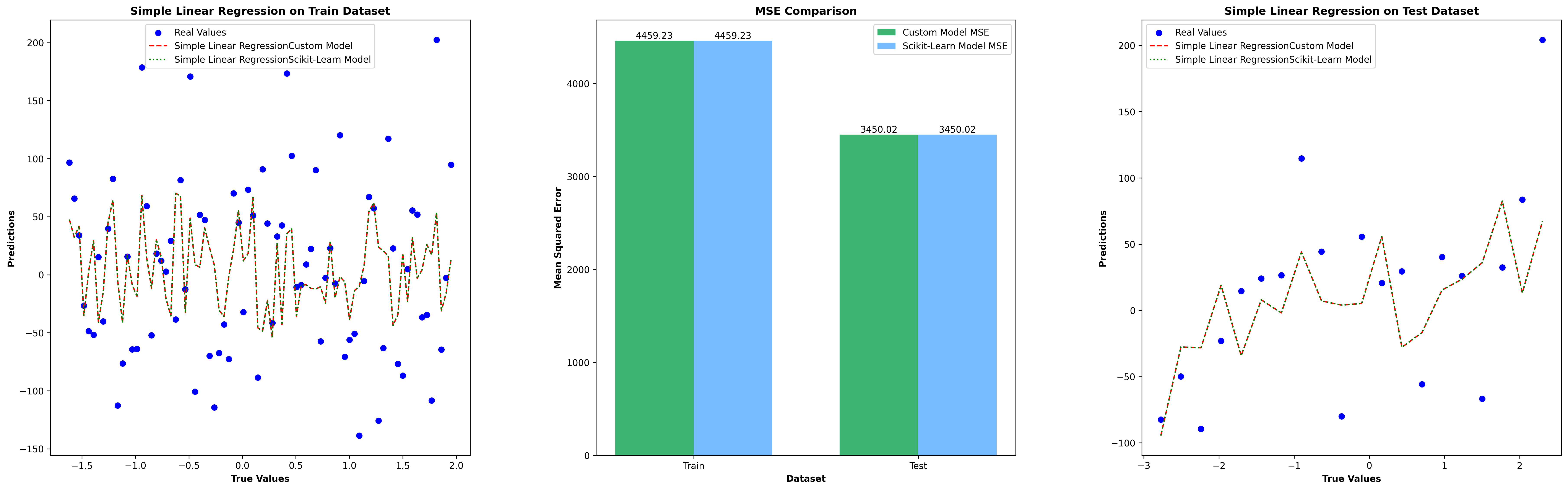Simple Linear Regression Test Results

from sklearn.linear_model import LinearRegression as SklearnLR

def test_simple_linear_regression(X_train,X_test,y_train,y_test,save_file=False):
    simple_reg = LinearRegressionCustom()
    simple_reg.fit(X_train[:, [0]], y_train)  

    y_pred_custom_train = simple_reg.predict(X_train[:, [0]])
    y_pred_custom_test = simple_reg.predict(X_test[:, [0]])
    sklearn_simple_reg = SklearnLR()
    sklearn_simple_reg.fit(X_train[:, [0]], y_train)
    
    y_pred_train_sklearn = sklearn_simple_reg.predict(X_train[:, [0]])
    y_pred_test_sklearn = sklearn_simple_reg.predict(X_test[:, [0]])
    
    evaluate_plot_results(X_train,y_train,y_pred_custom_train,y_pred_custom_test,X_test,y_test,y_pred_train_sklearn,y_pred_test_sklearn,title='Simple Linear Regression',save_file=save_file)

---

Multi-Linear Regression Test Results

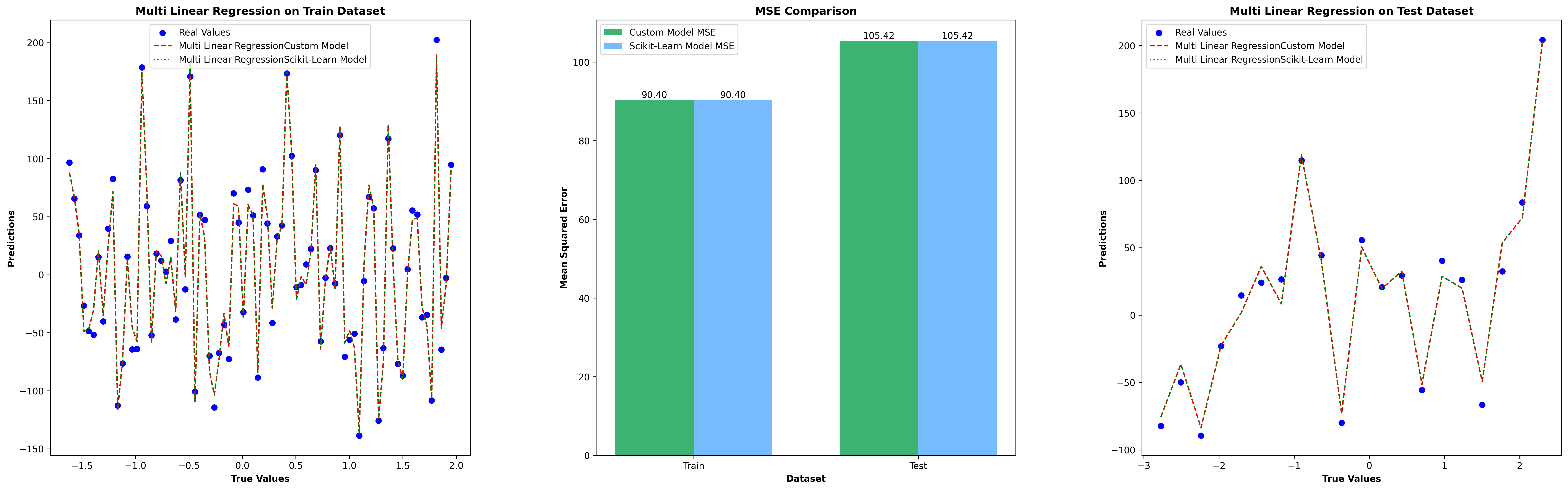Multi Linear Regression Test Results

from sklearn.linear_model import LinearRegression as SklearnLR

def test_multi_linear_regression(X_train,X_test,y_train,y_test,save_file=False):
    multi_reg = LinearRegressionCustom()
    multi_reg.fit(X_train, y_train)

    y_pred_custom_train = multi_reg.predict(X_train)
    y_pred_custom_test = multi_reg.predict(X_test)
    
    sklearn_multi_reg = SklearnLR()
    sklearn_multi_reg.fit(X_train, y_train)
    y_pred_train_sklearn = sklearn_multi_reg.predict(X_train)
    y_pred_test_sklearn = sklearn_multi_reg.predict(X_test)

    evaluate_plot_results(X_train,y_train,y_pred_custom_train,y_pred_custom_test,X_test,y_test,y_pred_train_sklearn,y_pred_test_sklearn,title='Multi Linear Regression',save_file=save_file)

---

Lasso Regression Test Results

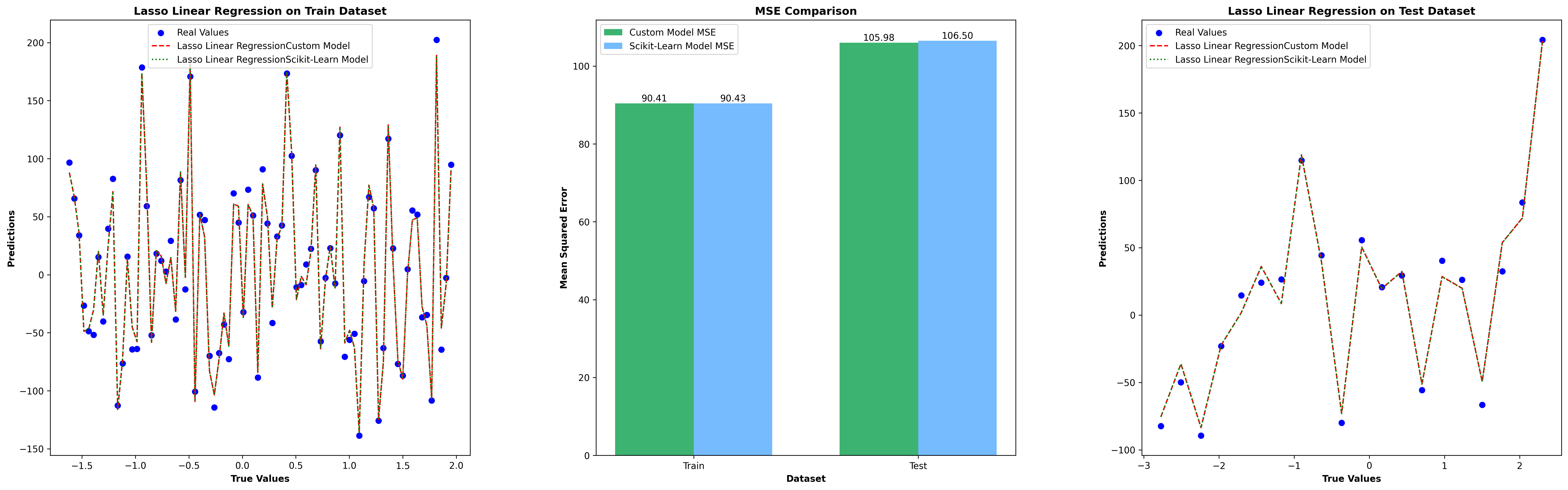Lasso Linear Regression Test Results

from sklearn.linear_model import Lasso

def test_lasso_linear_regression(X_train,X_test,y_train,y_test,save_file=False):
    lasso_reg = LinearRegressionCustom(alpha=0.1, lasso=True)
    lasso_reg.fit(X_train, y_train)
    # Predictions (Custom Implementation)
    y_pred_custom_train = lasso_reg.predict(X_train)
    y_pred_custom_test = lasso_reg.predict(X_test)
    
    # Fit models (Scikit-Learn)
    sklearn_lasso_reg = Lasso(alpha=0.1)
    sklearn_lasso_reg.fit(X_train, y_train)
    
    y_pred_train_sklearn = sklearn_lasso_reg.predict(X_train)
    y_pred_test_sklearn = sklearn_lasso_reg.predict(X_test)

    evaluate_plot_results(X_train,y_train,y_pred_custom_train,y_pred_custom_test,X_test,y_test,y_pred_train_sklearn,y_pred_test_sklearn,title='Lasso Linear Regression',save_file=save_file)

---

Ridge Regression Test Results

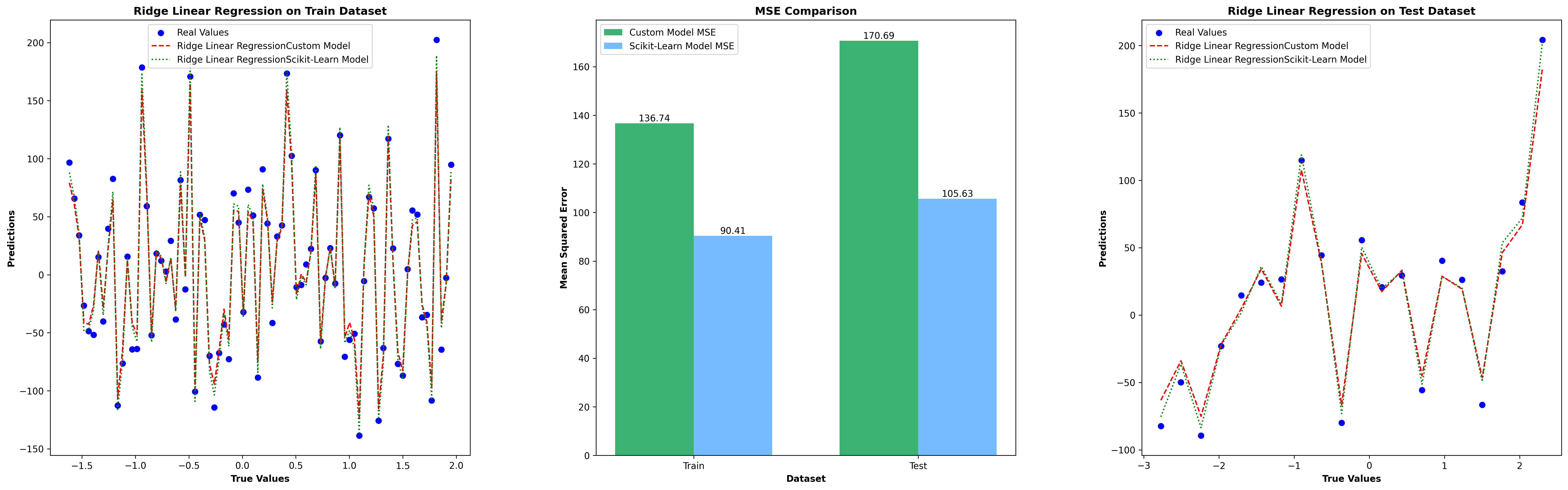Ridge Linear Regression Test Results

from sklearn.linear_model import Ridge

def test_ridge_linear_regression(X_train,X_test,y_train,y_test,save_file=False):
    ridge_reg = LinearRegressionCustom(alpha=0.1, ridge=True)
    ridge_reg.fit(X_train, y_train)
        
    y_pred_custom_train = ridge_reg.predict(X_train)
    y_pred_custom_test = ridge_reg.predict(X_test)
    sklearn_ridge_reg = Ridge(alpha=0.1)
    sklearn_ridge_reg.fit(X_train, y_train)

    y_pred_train_sklearn = sklearn_ridge_reg.predict(X_train)
    y_pred_test_sklearn = sklearn_ridge_reg.predict(X_test)
    evaluate_plot_results(X_train,y_train,y_pred_custom_train,y_pred_custom_test,X_test,y_test,y_pred_train_sklearn,y_pred_test_sklearn,title='Ridge Linear Regression',save_file=save_file)

---

Dataset & Evaluation Codes

from sklearn.datasets import make_regression
from sklearn.model_selection import train_test_split
from sklearn.metrics import mean_squared_error
import matplotlib.pyplot as plt 
from matplotlib.gridspec import GridSpec

def create_dataset() -> tuple:
    np.random.seed(0)
    X, y = make_regression(n_samples=100, n_features=3, noise=10, random_state=0)
    X_train, X_test, y_train, y_test = train_test_split(X, y, test_size=0.2, random_state=0)
    return X_train,X_test,y_train,y_test


def evaluate_plot_results(x_train,y_train, y_pred_train_custom, y_pred_test_custom, x_test,y_test, y_pred_train_sklearn, y_pred_test_sklearn,title,feature_idx=0,save_file=False):
    # Default check for first feature on features, because feature index parameter is 0. 
    
    # Calculate MSE
    mse_custom_train = mean_squared_error(y_train, y_pred_train_custom)
    mse_sklearn_train = mean_squared_error(y_train, y_pred_train_sklearn)
    mse_custom_test = mean_squared_error(y_test, y_pred_test_custom)
    mse_sklearn_test = mean_squared_error(y_test, y_pred_test_sklearn)
    
    fig = plt.figure(figsize=(30, 20))
    gs = GridSpec(2, 3, figure=fig)
    ax1 = fig.add_subplot(gs[0, 0])

    
    x_train_line = np.linspace(x_train[:,feature_idx].min(), x_train[:,feature_idx].max(), len(y_train)).reshape(-1, 1)
    
    # Scatter plot for train predictions
    ax1.scatter(x_train_line, y_train, color='blue', label='Real Values')
    ax1.plot(x_train_line,y_pred_train_custom, color='red', label=title + 'Custom Model',linestyle='--')
    ax1.plot(x_train_line,y_pred_train_sklearn, color='green', label=title + 'Scikit-Learn Model',linestyle=':')

    ax1.set_title(title + ' on Train Dataset',fontweight='bold')
    ax1.set_xlabel("True Values",fontweight='bold')
    ax1.set_ylabel("Predictions",fontweight='bold')
    ax1.legend()

    # Scatter plot for test predictions
    x_test_line = np.linspace(x_test[:,feature_idx].min(), x_test[:,feature_idx].max(),  len(y_test)).reshape(-1, 1)
    
    ax2 = fig.add_subplot(gs[0, 2])
    ax2.scatter(x_test_line, y_test, color='blue', label='Real Values')
    ax2.plot(x_test_line,y_pred_test_custom, color='red', label=title + 'Custom Model',linestyle='--')
    ax2.plot(x_test_line,y_pred_test_sklearn, color='green', label=title + 'Scikit-Learn Model',linestyle=':')
    ax2.set_title(title + ' on Test Dataset',fontweight='bold')
    ax2.set_xlabel("True Values",fontweight='bold')
    ax2.set_ylabel("Predictions",fontweight='bold')
    ax2.legend()

    # MSE comparison bar plot
    ax3 = fig.add_subplot(gs[0, 1])
    x = np.arange(2)  # position of the bars
    width = 0.35  # width of bars

    bars1 = ax3.bar(x - width/2, [mse_custom_train, mse_custom_test], width, label='Custom Model MSE', color='mediumseagreen')
    bars2 = ax3.bar(x + width/2, [mse_sklearn_train, mse_sklearn_test], width, label='Scikit-Learn Model MSE', color='xkcd:sky blue')

    # Add text for the bar heights
    for bar in bars1:
        height = bar.get_height()
        ax3.text(bar.get_x() + bar.get_width()/2.0, height, f'{height:.2f}', ha='center', va='bottom')

    for bar in bars2:
        height = bar.get_height()
        ax3.text(bar.get_x() + bar.get_width()/2.0, height, f'{height:.2f}', ha='center', va='bottom')

    ax3.set_xlabel('Dataset',fontweight='bold')
    ax3.set_ylabel('Mean Squared Error',fontweight='bold')
    ax3.set_title('MSE Comparison',fontweight='bold')
    ax3.set_xticks(x)
    ax3.set_xticklabels(['Train', 'Test'])
    ax3.legend()
    
    gs.update(hspace=.3, wspace=.3)
    if save_file:plt.savefig(title+'.png',dpi=300, bbox_inches='tight')
    else:plt.show()  

Classification

For binary classification, for example, we can set up a linear model as follows:

\[\hat{y} = w_0 x_0 + w_1 x_1 + \ldots + w_n x_n + b > 0\]

As seen, this formula closely resembles linear regression. However, it includes a threshold value. If the computed value is greater than 0, the model returns +1; otherwise, it returns -1. Linear models can be classified into different types based on the regularization algorithms and measurement metrics they use. The same applies to classification tasks. Two well-known methods are Logistic Regression and Support Vector Machines (SVMs). Logistic Regression

Despite the name, logistic regression should not be confused with regression methods. Logistic regression is a classification algorithm.

Problems have multiple features, one feature may be selected and the others separated for solving the problem.

Conclusion

"If you’re tackling a new problem and need a quick and effective tool, linear models are worth considering. They might not be the fanciest option, but they often provide a solid foundation for more complex models."