K-means Clustering
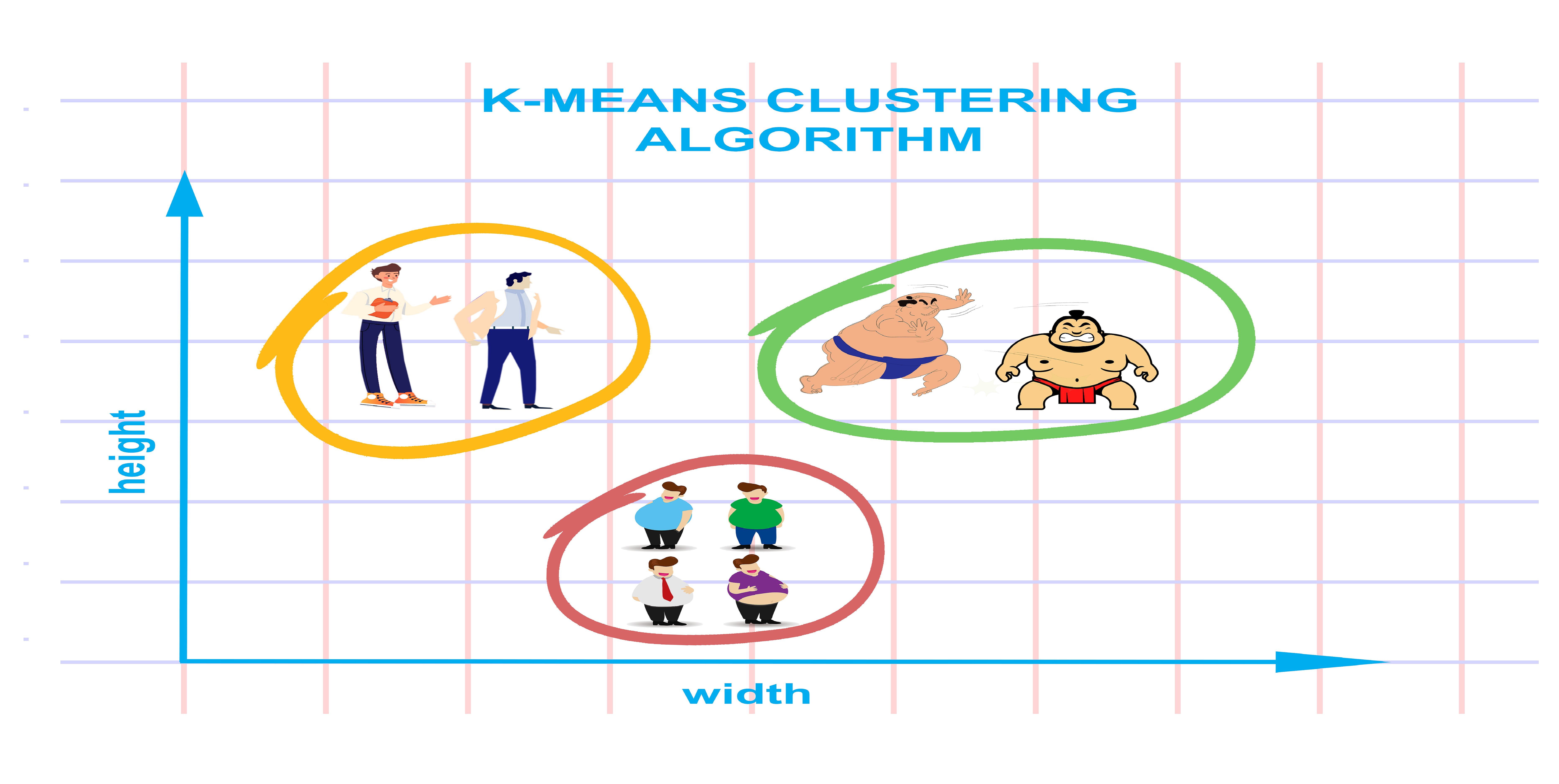
The K-Means algorithm is a popular clustering method in machine learning for grouping data points into clusters.
Understanding the K-Means Algorithm: A Simple Guide
The K-Means algorithm is a widely used method in machine learning for grouping data points into clusters. In this post, I’ll explain how it works, how to implement it, and how to evaluate its performance. I’ll also touch on some advantages and disadvantages of the K-Means algorithm and compare it to other clustering techniques.
What is K-Means?
At its core, K-Means is a way to group similar data points together. You tell the algorithm how many groups (or clusters) you want, and it will organize your data accordingly.
How Does K-Means Work?
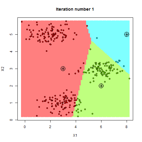 K-means Algorithm Process
Here’s a step-by-step breakdown of how K-Means clusters your data:
- Step—1 Choose K Initial Points: The algorithm starts by picking K random points from your data. These points act as the initial “centroids” or centers of the clusters.
- Step—2 Assign Data Points to Clusters: Each data point is assigned to the nearest centroid. This forms your initial clusters.
- Step—3 Update Centroids: The algorithm recalculates the centroids of these clusters based on the current members of each cluster.
- Step—4 Repeat: Steps 2 and 3 are repeated until the centroids no longer change significantly, meaning the clusters have stabilized.
The Math Behind K-Means
The K-Means algorithm tries to minimize the distance between data points and their assigned cluster centroids. This distance is usually measured using the Euclidean distance formula:
\[d(x_i, \mu_j) = \sqrt{\sum_{m=1}^{n} (x_{im} - \mu_{jm})^2}\]Where:
- \(x_i\) is a data point.
- \(μ_j\) is the centroid of the cluster.
- \(n\) is the number of features.
The goal is to minimize the total sum of squared errors:
\[J = \sum_{j=1}^{K} \sum_{i=1}^{N_j} \|x_i^{(j)} - \mu_j\|^2\]Implementing K-Means from Scratch
Here’s how you can write the K-Means algorithm as a Python class. This class allows you to customize things like the number of clusters (K) and how distances are calculated.
1
2
3
4
5
6
7
8
9
10
11
12
13
14
15
16
17
18
19
20
21
22
23
24
25
26
27
28
29
30
31
32
33
34
35
36
37
38
39
40
41
42
43
44
45
46
47
48
49
50
51
52
53
54
55
import numpy as np

class KMeansCustom:
    def __init__(self, K=3, distance_metric='euclidean', init='random', max_iters=300, tol=1e-4, random_state=None):
        self.K = K
        self.distance_metric = distance_metric
        self.init = init
        self.max_iters = max_iters
        self.tol = tol
        self.random_state = random_state

    def _init_kmeans_plus_plus(self, X):
        # K-Means++ Initialization
        n_samples, n_features = X.shape
        centroids = np.empty((self.K, n_features))
        # Choose the first centroid randomly
        centroids[0] = X[np.random.randint(n_samples)]

        # Compute the remaining centroids
        for k in range(1, self.K):
            distances = np.min(np.linalg.norm(X[:, np.newaxis] - centroids[:k], axis=2), axis=1)
            probabilities = distances / distances.sum()
            next_centroid = X[np.random.choice(n_samples, p=probabilities)]
            centroids[k] = next_centroid

        return centroids

    def fit(self, X):
        np.random.seed(self.random_state)

        # K-Means++ Initialization
        if self.init == 'kmeans++':
            centroids = self._init_kmeans_plus_plus(X)
        else:
            # Random initialization
            centroids = X[np.random.choice(X.shape[0], self.K, replace=False)]

        labels = np.zeros(X.shape[0])
        for _ in range(self.max_iters):
            # Compute distances
            distances = np.linalg.norm(X[:, np.newaxis] - centroids, axis=2)
            # Assign labels based on closest centroid
            new_labels = np.argmin(distances, axis=1)

            # Recompute centroids
            new_centroids = np.array([X[new_labels == k].mean(axis=0) for k in range(self.K)])

            # Check for convergence
            if np.all(np.linalg.norm(new_centroids - centroids, axis=1) < self.tol):
                break

            labels = new_labels
            centroids = new_centroids

        return centroids, labels
Evaluating the Performance of K-Means
Evaluating how well K-Means performed is crucial. Here are some common methods:
- Inertia: This measures how tightly the data points are clustered around the centroids. Lower inertia indicates better clustering.
- Silhouette Score: This score shows how similar each data point is to its own cluster compared to other clusters. Scores close to 1 mean better clustering.
The Silhouette Score is calculated as:
\[S(i) = \frac{b(i) - a(i)}{\max\{a(i), b(i)\}}\]Where:
- \(a(i)\) is the average distance between a data point and all other points in the same cluster.
- \(b(i)\)b is the average distance between a data point and the points in the nearest different cluster.
Custom KMeans Model Test
1
2
3
4
5
6
7
8
9
10
11
12
13
14
15
16
17
18
19
20
21
22
23
24
25
26
27
28
29
30
31
32
33
34
35
36
37
from sklearn.datasets import make_blobs

# Generate synthetic data
X, y = make_blobs(n_samples=500, centers=5, cluster_std=0.70, random_state=42)

from sklearn.metrics import silhouette_score, davies_bouldin_score
import matplotlib.pyplot as plt

# Train the KMeans model
kmeans_random = KMeansCustom(K=5, init='random', max_iters=300, tol=1e-4, random_state=42)
centroids, labels = kmeans_random.fit(X)

# Calculate evaluation metrics
sil_score = silhouette_score(X, labels)
db_score = davies_bouldin_score(X, labels)

# Plot the clustering results with legends
plt.figure(figsize=(10, 6))
scatter = plt.scatter(X[:, 0], X[:, 1], c=labels, cmap='viridis', alpha=0.8, edgecolors='w', s=50)

# Add centroid points
plt.scatter(centroids[:, 0], centroids[:, 1], s=200, c='red', marker='X', label='Centroids')

# Add legend for clusters
unique_labels = np.unique(labels)
for label in unique_labels:
    plt.scatter([], [], color=plt.cm.viridis(label / max(labels)), label=f'Cluster {label + 1}')

plt.title('K-Means Clustering with Custom Model')
plt.xlabel('Feature 1')
plt.ylabel('Feature 2')
plt.legend()
plt.colorbar(scatter, label='Cluster')
plt.show()

print(f"Silhouette Score: {sil_score:.3f}")
print(f"Davies-Bouldin Score: {db_score:.3f}")
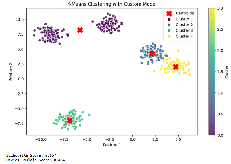 Custom K-means Model Test Results
Implementing K-Means with Scikit-Learn
Here’s how you can use Scikit-learn’s built-in K-Means function and evaluate its performance.
1
2
3
4
5
6
7
8
9
10
11
12
13
14
15
16
17
18
19
20
21
22
23
24
25
26
27
28
29
30
31
from sklearn.cluster import KMeans
# Train the KMeans model
kmeans = KMeans(n_clusters=4,max_iter=100,tol=1e-4,random_state=42)
kmeans.fit(X)
labels = kmeans.labels_
centroids = kmeans.cluster_centers_

# Calculate evaluation metrics
sil_score = silhouette_score(X, labels)
db_score = davies_bouldin_score(X, labels)

# Plot the clustering results with legends
plt.figure(figsize=(10, 6))
scatter = plt.scatter(X[:, 0], X[:, 1], c=labels, cmap='viridis', alpha=0.8, edgecolors='w', s=50)

# Add centroid points
plt.scatter(centroids[:, 0], centroids[:, 1], s=200, c='red', marker='X', label='Centroids')

# Add legend for clusters
unique_labels = np.unique(labels)
for label in unique_labels:
    plt.scatter([], [], color=plt.cm.viridis(label / max(labels)), label=f'Cluster {label + 1}')

plt.title('K-Means Clustering with Legends')
plt.xlabel('Feature 1')
plt.ylabel('Feature 2')
plt.legend()
plt.colorbar(scatter, label='Cluster')
plt.show()
print(f"Silhouette Score: {sil_score:.3f}")
print(f"Davies-Bouldin Score: {db_score:.3f}")
Scikit-Learn K-means Model Test
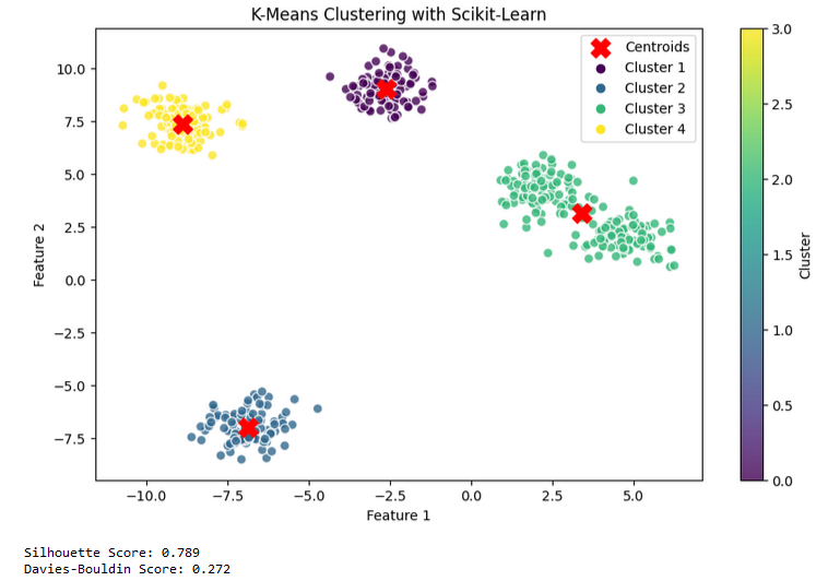 Scikit-learn K-means Model Test Results
The Elbow Method
The Elbow Method is used to determine the optimal number of clusters for K-Means. It involves plotting the inertia (or sum of squared distances from points to their assigned centroids) against different values of K. The “elbow” point in the plot, where the rate of decrease sharply changes, indicates the optimal number of clusters. With the Python code below, the optimal k was determined using the inertia and elbow method, and a code was written to calculate the optimal k according to the maximum silhouette score.
Implementing the Elbow Method
Here’s how you can use the Elbow Method to find the best K:
1
2
3
4
5
6
7
8
9
10
11
12
13
14
15
16
17
18
19
20
21
22
23
24
25
26
27
28
29
30
31
32
33
34
35
36
37
38
39
40
41
42
43
44
45
46
47
48
49
50
51
52
53
54
55
56
57
58
59
60
61
62
63
64
from kneed import KneeLocator #pip install kneed

# Compute KMeans for a range of K values and store inertia and silhouette scores
inertia = []
silhouette_scores = []
K_range = range(1, 11)

for K in K_range:
    kmeans = KMeans(n_clusters=K, random_state=42)
    kmeans.fit(X)
    inertia.append(kmeans.inertia_)
    if K > 1:  # Silhouette score is not defined for K=1
        labels = kmeans.labels_
        silhouette_scores.append(silhouette_score(X, labels))
    else:
        silhouette_scores.append(None)  # Placeholder for K=1

# Convert inertia and silhouette_scores to numpy arrays for further processing
inertia = np.array(inertia)
silhouette_scores = np.array(silhouette_scores)

# Apply Kneedle Algorithm to find the optimal K based on inertia
kneedle = KneeLocator(K_range, inertia, curve='convex', direction='decreasing')
optimal_k_inertia = kneedle.elbow

# Find the optimal K based on silhouette scores
optimal_k_silhouette = K_range[np.argmax(silhouette_scores[1:]) + 1]  # Skip K=1 for silhouette scores

# Plot the Elbow Method with Kneedle Detection, Silhouette Scores, and Optimal K
fig, ax1 = plt.subplots(figsize=(12, 6))

# Plot Inertia
color = 'tab:blue'
ax1.set_xlabel('Number of Clusters (K)')
ax1.set_ylabel('Inertia', color=color)
ax1.plot(K_range, inertia, marker='o', linestyle='-', color=color, markersize=8, linewidth=2, label='Inertia')
ax1.tick_params(axis='y', labelcolor=color)

# Plot Silhouette Scores
ax2 = ax1.twinx()  # Instantiate a second y-axis that shares the same x-axis
color = 'tab:red'
ax2.set_ylabel('Silhouette Score', color=color)  # We already handled the x-label with ax1
ax2.plot(K_range[1:], silhouette_scores[1:], marker='o', linestyle='--', color=color, markersize=8, linewidth=2, label='Silhouette Score')
ax2.tick_params(axis='y', labelcolor=color)

# Highlight the optimal K points
ax1.scatter(optimal_k_inertia, inertia[optimal_k_inertia - 1], color='black', s=100, edgecolor='black', zorder=5)
ax1.annotate(f'Optimal K (Inertia) = {optimal_k_inertia}',
             xy=(optimal_k_inertia, inertia[optimal_k_inertia - 1]),
             xytext=(optimal_k_inertia + 1, inertia[optimal_k_inertia - 1] + 1000),
             arrowprops=dict(facecolor='black', shrink=0.05),
             fontsize=12, color='black')

ax1.scatter(optimal_k_silhouette, inertia[optimal_k_silhouette - 1], color='green', s=100, edgecolor='black', zorder=5)
ax1.annotate(f'Optimal K (Silhouette) = {optimal_k_silhouette}',
             xy=(optimal_k_silhouette, inertia[optimal_k_silhouette - 1]),
             xytext=(optimal_k_silhouette + 1, inertia[optimal_k_silhouette - 1] + 1000),
             arrowprops=dict(facecolor='green', shrink=0.05),
             fontsize=12, color='green')

fig.tight_layout()  # Adjust layout to fit both y-axes
plt.title('Elbow Method with Kneedle Detection, Silhouette Scores, and Optimal K')
plt.grid(True)
plt.show()
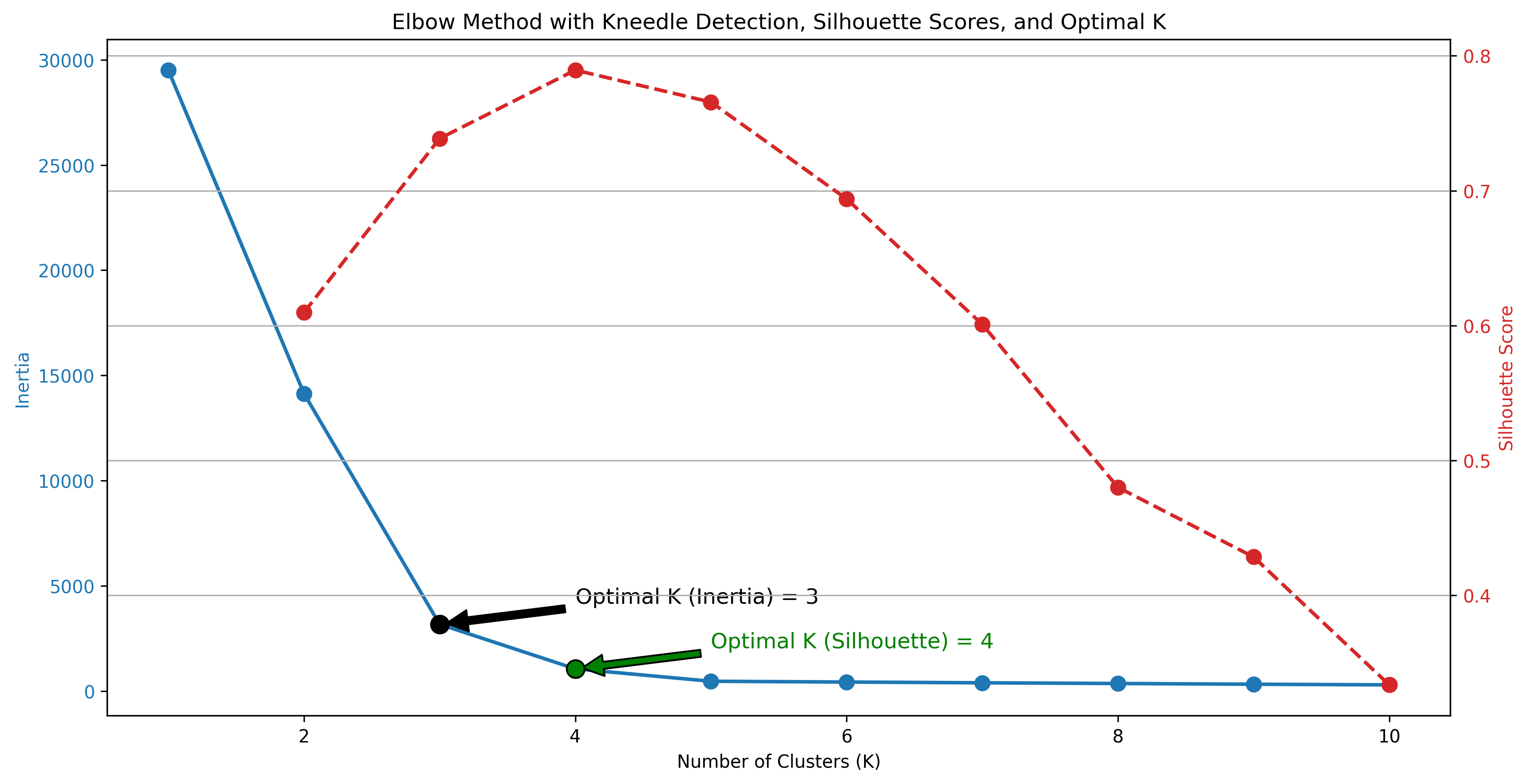 Elbow Method
Advantages and Disadvantages of K-Means
Advantages:
- Simplicity: Easy to understand and implement.
- Scalability: Works well with large datasets.
- Speed: Fast and efficient for clustering.
Disadvantages:
- Sensitivity to Initial Centroids: The final clusters can depend heavily on the initial centroids.
- Assumes Spherical Clusters: K-Means assumes that clusters are spherical, which might not always be true.
- Fixed Number of Clusters: You must decide the number of clusters (K) beforehand.
Conclusion
K-Means is a powerful tool for grouping and understanding your data. You can implement this algorithm from scratch using a class structure or use the Scikit-learn library to bring it to life. As can be seen from the results above, the k means algorithm in scikit-learn is better than the custom kmeans when we look at both the silhouette score and the davies bouldin score, so it would be better to use the model that we will call from scikit-learn for kmeans.Also selecting the right hyperparameters can significantly impact the algorithm’s performance, so it’s essential to use evaluation methods to measure your model’s success.
However, K-Means has its limitations. For example, it assumes that clusters are spherical and equally sized, which may not always be true in real-world data. Additionally, K-Means is sensitive to the initial placement of centroids, which can lead to different results on different runs.
For better clustering results, you might want to consider other algorithms, such as:
- Hierarchical Clustering: Suitable for creating a hierarchy of clusters, especially when you don’t know the number of clusters beforehand.
- DBSCAN (Density-Based Spatial Clustering of Applications with Noise): Effective in finding clusters of arbitrary shape and handling noise in the data.
- Gaussian Mixture Models (GMM): Provides a probabilistic approach to clustering, allowing for clusters of different shapes and sizes.
Each of these alternatives can offer better performance depending on the characteristics of your data. By understanding and applying the right clustering algorithm, you can unlock deeper insights from your data.