Your Friendly Neighborhood Algorithm is KNN
The k-Nearest Neighbors (KNN) algorithm is like asking your friends for advice based on who’s closest to you. It figures out your data's category by looking at its nearest neighbors and deciding which ones matter most.
Introduction
I am sure many of us have heard the following expression in our daily life; Tell me about your friend and I will tell you who you are. Likewise, the k-nearest neighbor algorithm uses other points around it to define data points. k-Nearest Neighbours (KNN) algorithm is one of the supervised learning algorithms. It works with labeled data just like any other supervised algorithm. It establishes a relationship between labeled data and unlabeled data through their neighborhood and distance to them. The KNN algorithm can be diversified in three different ways: Number of Neighborhoods (k) : We can specify how many of the surrounding data (points) we will associate with. (k = 2,3,5 etc.) Distance Calculation Method: With which distance method can we examine the relationship with the surrounding data (Euclidean, Manhattan, Minkowski, Chebyshev etc.) Equal Relationship Instant Decision Method: What method will the relationship be terminated when the relationship rate with the surrounding points is equal? (randomness or select first etc.)
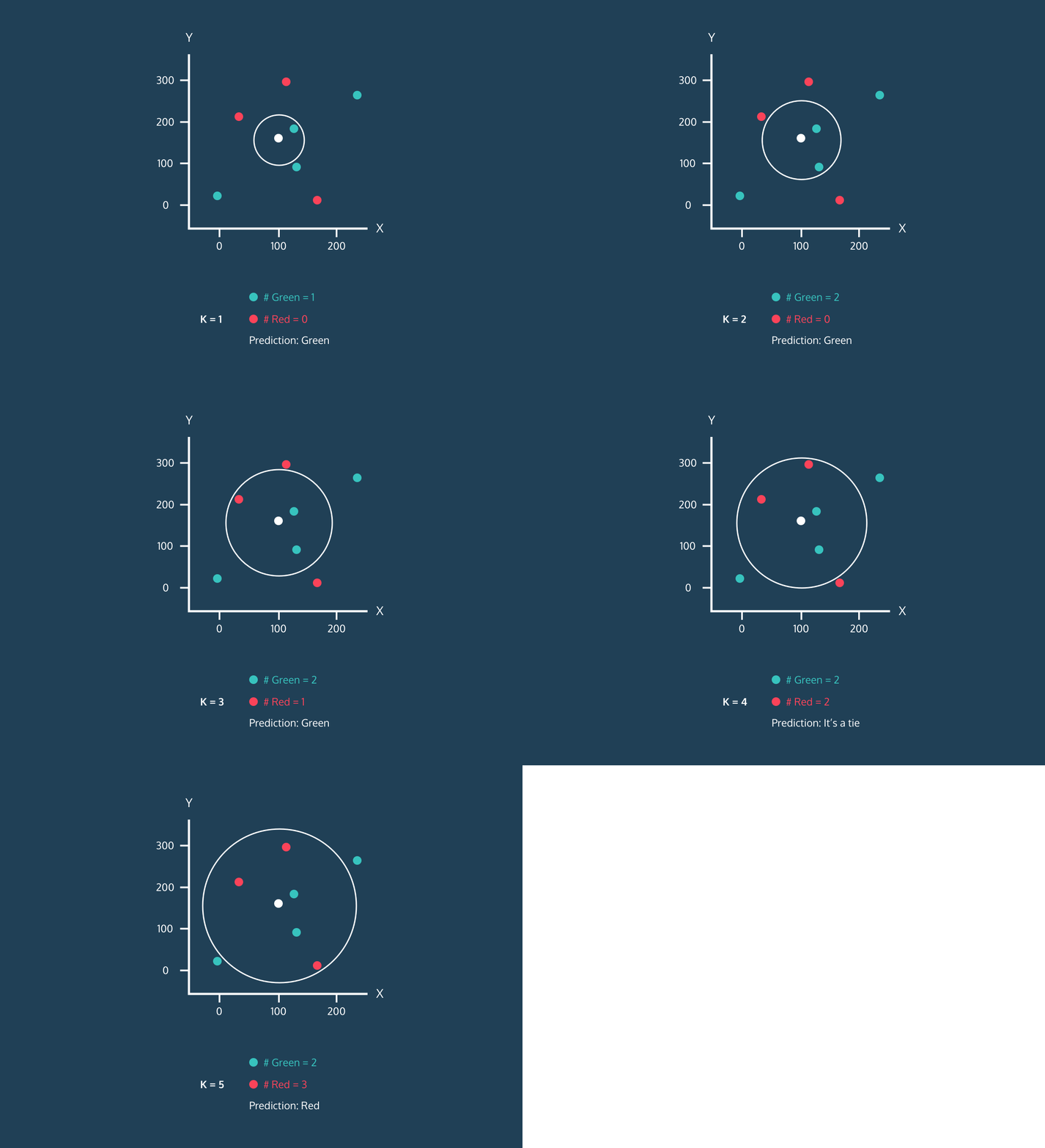
 Image 1. KNN Algorithm Demo for a Single White Dot.Image by Datacamp
Algorithm Steps
A demo of the KNN Algorithm for a single point is performed on Figure 1. Before we move on to this demo, it would be helpful to know algorithm:
- Step 1 — While creating the algorithm, definitions are made with which method the algorithm will calculate the distances between the points and how many nearby points it will look at.
- Step 2 — Labeled data and unlabeled data to be predicted are loaded into or trained by the algorithm, which we call the fit step.
- Step 3 — The distances between each point in the data to be estimated and the labeled data are calculated.
- Step 4 — According to the calculations, the distances are sorted from smallest to largest, that is, from near to far.
- Step 5 — In this order, the number of neighbors we use while defining the algorithm is looked at as well as its neighbors, that is, the points near it. Unlabeled data is labeled according to the label of the number of points that have a majority among these points. If there is equality, a random selection can be made.
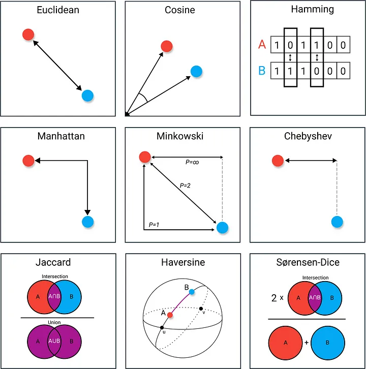
Let’s assume that the distance calculation method in the first step is defined in the demo in Figure 1. Besides at this point, I would like to share with you a nice visual and article about the distance calculation methods that can be used.
 Image 2. Distance Methods. Image by Maarten Grootendorst
Okay let’s continue to Figure 1 , in the continuation of first step, we need to determine the number of neighbors. As seen in the demo, our estimation changes as the number of neighbors changes. Even at a time when it has equal neighbors, the algorithm enters a tie. At this point, we can have our algorithm randomly choose or choose the first label it sees. Also, in the example in the 3rd figure below, we want to predict whether a new point will be red or blue in a knn algorithm that will look at 3 neighborhoods. Since this black dot is close to 1 blue and 2 red dots, it is labeled as red because the majority are red dots.
 Image 3. KNN Classification for K=3 | 1 blue < 2 red | new point is red. Image by Gfycat </a>
Advantages and Disadvantages
The KNN Algorithm is advantageous in terms of being quickly set up, implemented and explained. However, it is a costly algorithm in terms of time and space. Calculating the distance of a point from all other points in the dataset is a costly task. Curse of dimensionality can occur, especially when working with high-dimensional data. For this reason, many people use it with small data sets, but it is not recommended to be used with large data sets.
Let’s code this algorithm from scratch with the iris dataset that most of us know.
Step by Step KNN Code
Step 1 - Initalize Neighbour count and distance method.
1
2
3
4
5
6
7
8
9
10
11
12
13
14
15
16
class KNearestNeighbours:
  def __init__(self,k=5,distance_method='euclidean'):
      self.neighbour_count = k
      self.distance_method = distance_method

  def set_neighbour_count(self,k:int) -> None:
      self.neighbour_count = k

  def get_neighbour_count(self)->int:
      return self.neighbour_count

  def set_distance_method(self,distance_method:str) -> None:
      self.distance_method = distance_method

  def get_distance_method(self)->str:
      return self.distance_method
Step 2 - Fit the Algorithm with Training Data
1
2
3
def fit(self,x:np.array,y:np.array):
  self.X_train = x
  self.y_train = y
Step 3 - Calculate Distance Between Points
1
2
3
4
5
6
7
8
9
10
11
12
from scipy.spatial import distance

def __calculate_distance(self,u:np.array,v:np.array) -> float:
  methods = {
      'euclidean':distance.euclidean(u,v),
      'minkowski':distance.minkowski(u,v),
      'manhattan':distance.cityblock(u,v),
      'chebyshev':distance.chebyshev(u,v),
      'jaccard':distance.jaccard(u,v),
      'cosine': distance.cosine(u,v),
      }
  return methods[self.distance_method]
Step 4 & Step 5- Sort Distances and Select k Nearest Points
1
2
3
4
5
6
7
8
9
10
11
12
13
14
15
16
17
18
19
20
21
22
23
24
from collections import Counter

def __predict(self,x_pred:np.array):
  # step 3
  distances = [self.__calculate_distance(x_pred,x_real) for x_real in self.X_train]

  # step 4
  sorted_distances_as_idx = np.argsort(distances)
  knn_indices = sorted_distances_as_idx[:self.neighbour_count]
  predicted_values = self.y_train[knn_indices].squeeze().tolist()

  # step 5
  most_common_values = Counter(predicted_values).most_common()
  prediction = most_common_values[0][0]
  return prediction

  #Function that is below is apply step 4 & step 5 for all test data points.
  def predict(self,X_test:np.array) -> list:
    if X_test.ndim == 1:
        X_test = np.expand_dims(X_test,axis=0)

    predictions = [self.__predict(x_pred) for x_pred in X_test]
    return predictions
Test on Iris Dataset
Let’s test this module with iris dataset using scikit-learn. The iris dataset can be easily loaded from scikit-learn. It basically consists of 5 columns, 4 feature and 1 target column. Let’s convert the dataset to pd.DataFrame using scikit-learn, NumPy and Pandas.
1
2
3
4
5
6
7
8
9
10
11
12
13
14
15
16
17
18
19
20
21
22
23
24

from sklearn.datasets import load_iris
from sklearn.model_selection import train_test_split
import numpy as np
import pandas as pd

dataset = load_iris()

data = np.concatenate((dataset.data,dataset.target.reshape(-1,1)),axis=1)
columns = dataset.feature_names + ['class']
# cols:'sepal length (cm), sepal width (cm), petal length (cm), petal width (cm), class'

df = pd.DataFrame(data=data,columns=columns)

class_map = dict(enumerate(dataset.target_names))
# class_map = {0: 'setosa', 1: 'versicolor', 2: 'virginica'}

df['class_name'] = df['class'].apply(lambda v:class_map[int(v)])
df = df.sample(frac = 1) # shuffle dataset
df = df.reset_index(drop=True) # reset index on shuffled data

# Train Test Split
X,y = df.iloc[:,:-2],df.iloc[:,-2]
X_train,X_test,y_train,y_test = train_test_split(X,y,random_state=42,test_size=0.1)
 First 5th Rows of the Dataframe [ df.head( ) ]
Let’s create and fit our k-Nearest Neighbours model. Then, predict test data with the model. Finally, let’s calculate the accuracy.
1
2
3
4
knn = KNearestNeighbours(k=3,distance_method='euclidean')
knn.fit(x=X_train.values,y=y_train.values)
predictions = knn.predict(X_test=X_test.values)
acc = np.sum(predictions == y_test.values) / len(y_test)
 Results of Our Training & Prediction
Full Code
1
2
3
4
5
6
7
8
9
10
11
12
13
14
15
16
17
18
19
20
21
22
23
24
25
26
27
28
29
30
31
32
33
34
35
36
37
38
39
40
41
42
43
44
45
46
47
48
49
50
51
52
53
54
55
56
57
58
59
60
61
62
63
64
65
66
67
68
69
70
71
72
73
74
75
76
from scipy.spatial import distance
from collections import Counter
from sklearn.datasets import load_iris
from sklearn.model_selection import train_test_split
import numpy as np
import pandas as pd

class KNearestNeighbours:
    def __init__(self,k=5,distance_method='euclidean'):
        self.neighbour_count = k
        self.distance_method = distance_method

    def set_neighbour_count(self,k:int) -> None:
        self.neighbour_count = k

    def get_neighbour_count(self)->int:
        return self.neighbour_count

    def set_distance_method(self,distance_method:str) -> None:
        self.distance_method = distance_method

    def get_distance_method(self)->str:
        return self.distance_method

    def fit(self,x:np.array,y:np.array):
        self.X_train = x
        self.y_train = y

    def __calculate_distance(self,u:np.array,v:np.array) -> float:
        methods = {
            'euclidean':distance.euclidean(u,v),
            'minkowski':distance.minkowski(u,v),
            'manhattan':distance.cityblock(u,v),
            'chebyshev':distance.chebyshev(u,v),
            'jaccard':distance.jaccard(u,v),
            'cosine': distance.cosine(u,v),
            }
        return methods[self.distance_method]


    def __predict(self,x_pred:np.array):
        distances = [self.__calculate_distance(x_pred,x_real) for x_real in self.X_train]
        sorted_distances_as_idx = np.argsort(distances)
        knn_indices = sorted_distances_as_idx[:self.neighbour_count]
        predicted_values = self.y_train[knn_indices].squeeze().tolist()
        most_common_values = Counter(predicted_values).most_common()
        prediction = most_common_values[0][0]
        return prediction

    def predict(self,X_test:np.array) -> list:
        if X_test.ndim == 1:
            X_test = np.expand_dims(X_test,axis=0)

        predictions = [self.__predict(x_pred) for x_pred in X_test]
        return predictions

dataset = load_iris()

data = np.concatenate((dataset.data,dataset.target.reshape(-1,1)),axis=1)
columns = dataset.feature_names + ['class']

df = pd.DataFrame(data=data,columns=columns)
class_map = dict(enumerate(dataset.target_names))

df['class_name'] = df['class'].apply(lambda v:class_map[int(v)])
df = df.sample(frac = 1)
df = df.reset_index(drop=True)

# Train Test Split
X,y = df.iloc[:,:-2],df.iloc[:,-2]
X_train,X_test,y_train,y_test = train_test_split(X,y,random_state=42,test_size=0.1)

knn = KNearestNeighbours(k=3,distance_method='euclidean')
knn.fit(x=X_train.values,y=y_train.values)
predictions = knn.predict(X_test=X_test.values)
acc = np.sum(predictions == y_test.values) / len(y_test)
Conclusion
The k-Nearest Neighbors (KNN) algorithm is like the friendly neighbor who knows everyone in the neighborhood. By examining the closest "neighbors" to a data point, KNN makes predictions based on the characteristics of these nearby data points. This approach offers several advantages, such as simplicity and ease of implementation. However, it’s essential to be aware of its limitations, including sensitivity to noisy data and the computational cost associated with large datasets. Despite these challenges, KNN remains a valuable tool when used with care.
