Decision Trees | Growing Your Way to Smarter Decisions
Decision trees are a foundational tool in machine learning, offering a clear and intuitive method for both classification and regression tasks. This guide provides a detailed exploration of decision trees, from their core concepts to practical implementation.

Introduction to Decision Trees
Decision trees are one of the most popular and widely used algorithms in machine learning, particularly for classification and regression tasks. They belong to the family of supervised learning algorithms and work by splitting the data into smaller subsets based on certain criteria. The result is a tree-like model of decisions that leads to a final output (label). This structure resembles the flow of decisions and their possible outcomes, hence the name “decision tree.”
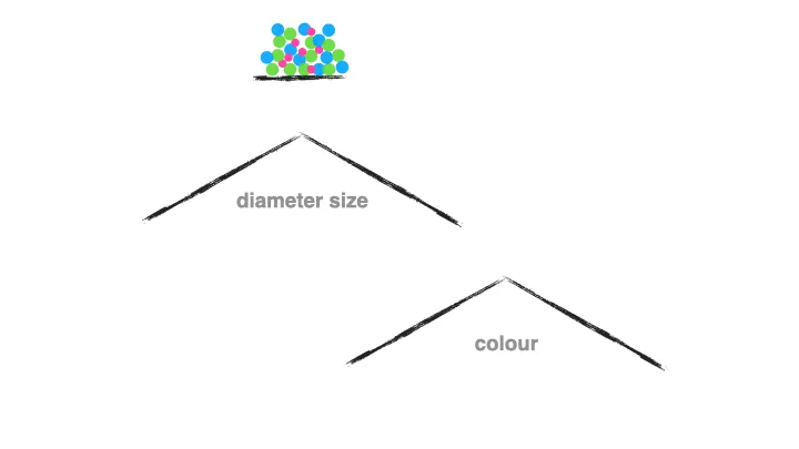 Dataset Split in a Decision Tree. Image by ml2gifs
The key idea behind decision trees is to select the best feature at each node to partition the data into subsets that are as homogenous as possible. This process is repeated recursively for each subset until the stopping criteria are met, either when the maximum depth is reached or when the data cannot be split any further.
Let’s say you are trying to decide what to wear. Your decision tree might ask: “Is it raining?” If yes, you grab an umbrella. If not, it might ask: “Is it cold?” and so on, until you have decided on your outfit for the day. In machine learning, decision trees do the same thing but with data, and instead of picking outfits, they are making predictions or classifications.
Why Should You Care About Decision Trees?
Ever tried explaining deep learning models to a non-techie friend? Yeah, not easy. But decision trees? They are a breeze to explain. You can see the decisions being made right in front of you, like following a flowchart. This makes them incredibly interpretable — you can understand exactly why the model made a particular prediction, which is super handy when you are working with stakeholders who demand transparency.
Another perk? Decision trees do not care about whether your data is on the same scale or even if it is numerical or categorical. Whether you are dealing with temperatures or zip codes, decision trees handle it all. Plus, they are great at dealing with complex, non-linear relationships. If there is a twisty path through the data, they will find it!
When to Use Decision Trees?
- You need something easy to explain: They are perfect for building models that both you and your team can understand and explain to others.
- Your data has both numbers and categories: Trees handle both seamlessly, so you do not need to spend time converting everything to the same format.
- You suspect there is a complex relationship hiding in your data: Trees will dig deep, splitting your data at every opportunity to find those hidden patterns.
Overview of Decision Trees
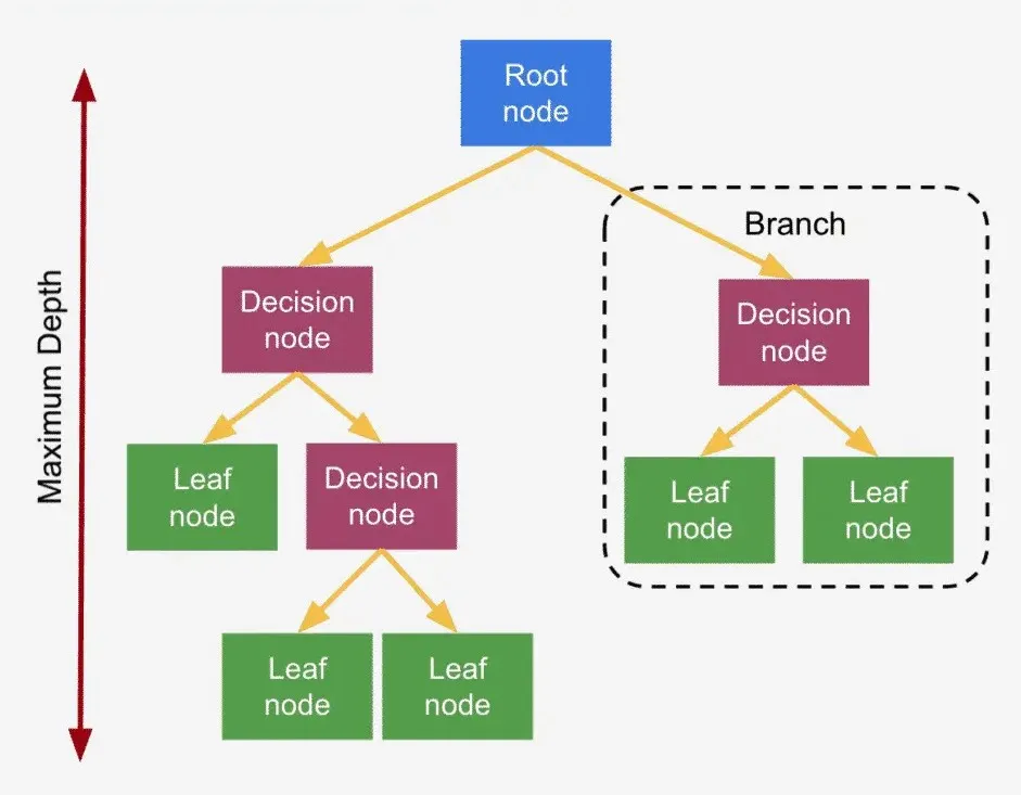 Decision Tree Structure
In a decision tree, each decision(internal) node represents a test or condition on a feature (e.g., “Is Feature 1 greater than 5?”), each branch represents the outcome of that condition, and each leaf node represents a class label or final decision. The algorithm splits data by selecting the feature and threshold that provides the highest information gain (or lowest impurity).
Common Splitting Criteria:
\[G(D) = 1 - \sum_{i=1}^c p_i^2\]
- Gini Index: Measures the degree of probability of a particular feature being classified incorrectly when randomly chosen.
\[H(D) = - \sum_{i=1}^c p_i \log_2(p_i)\] \[\text{Information Gain}(D, \text{split}) = H(D) - \left( \frac{|D_{\text{left}}|}{|D|} H(D_{\text{left}}) + \frac{|D_{\text{right}}|}{|D|} H(D_{\text{right}}) \right)\]
- Entropy : Measures the amount of uncertainty or disorder in the data, aiming to reduce uncertainty with each split.
In these formulas:
- $p_i$ represents the proportion of samples belonging to class ii.
- $c$ is the number of classes.
- $∣D_{left}∣$ and $∣D_{right}∣$ denote the number of samples in the left and right subsets, respectively.
- $H(D)$, $H(D_{left})$, and $H(D_{right})$ are the entropies or Gini impurities before and after the split.
Pros and Cons of Decision Trees
Advantages
- Crystal clear: The decisions are laid out in a way that anyone can follow.
- Flexibility: Trees work well with both numbers and categories, and you don’t need to do a ton of data prep beforehand.
- Handles complexity: Trees can capture complex relationships that simpler models might miss.
Disadvantages
- Overfitting danger: If you let the tree grow too deep, it starts to memorize the data rather than learn from it—kind of like a detective who sees conspiracies everywhere. Pruning the tree or limiting its depth helps prevent this.
- A bit fickle: Small changes in the data can sometimes result in a totally different tree, which makes them less stable than other models.
- Bias risk: Trees can sometimes get obsessed with features that have many levels or categories, ignoring others that might be more important.
Building a Decision Tree from Scratch: Step-by-Step
Let’s dive into the algorithm to build a decision tree from scratch using the Python code provided.
1. Initialize the Tree
We start by creating a Node class that will represent each node in the decision tree. Each node will store important information such as the feature index, threshold for splitting, and pointers to left and right child nodes.In otherwords, this node is like a fork in the road—it holds the feature we’re asking about and which way we’ll go based on the answer.
1
2
3
4
5
6
7
8
9
10
11
class Node:
    def __init__(self,feature_index=None,threshold=None,condition_mark=None,left=None,right=None,score=None,criterion=None,information_gain=None,label=None):
        self.feature_index = feature_index
        self.threshold = threshold
        self.condition_mark = condition_mark
        self.left = left
        self.right = right
        self.score = score
        self.criterion = criterion
        self.information_gain = information_gain
        self.label = label
2. Stopping Conditions
Before splitting the data, we check whether we should stop further splitting. This can happen if the data at the node is pure (contains only one class) or if the maximum depth or minimum samples condition is met.
1
2
3
4
5
def _should_stop(self,data,depth):
    n_labels = len(np.unique(data[:,-1]))
    n_samples = len(data)
    condition = (n_labels == 1) or (n_samples <= self.min_samples_count) or (depth >= self.max_depth)
    return condition
3. Splitting the Data
At each node, we calculate potential splits for both categorical and numerical features. For numerical features, we use the median as a threshold, while for categorical features, we split by unique values.
1
2
3
4
5
6
7
8
9
10
11
12
13
def _get_potential_splits(self,data):
    potential_splits_all = []
    n_features = data.shape[1] - 1  # [feat_1, feat_2, ..., feat_n, labels]
    for feature_idx in range(n_features):
        data_feature = data[:,feature_idx]
        if isinstance(data_feature[0],str) or isinstance(data_feature[0],bool):
            thresholds = np.unique(data_feature)
            condition_mark = '=='
        else:
            thresholds = [np.median(data_feature)]
            condition_mark = '<='
        potential_splits_all.append({'idx':feature_idx,'thresholds':thresholds,'condition_mark':condition_mark})
    return potential_splits_all
4. Calculating Information Gain
Next, we evaluate the information gain for each potential split. The information gain tells us how much uncertainty is reduced after splitting the data. We choose the split that provides the highest information gain.
1
2
3
4
5
6
7
def _calculate_information_gain(self,labels, left_idxs, right_idxs):
    p_left = len(left_idxs) / len(labels)
    p_right = 1 - p_left
    weighted_impurity = p_left * self._calculate_impurity(labels[left_idxs]) + p_right * self._calculate_impurity(labels[right_idxs])
    parent_impurity = self._calculate_impurity(labels)
    information_gain = parent_impurity - weighted_impurity
    return information_gain, weighted_impurity
5. Recursive Tree Building
Using the best split found, we recursively build the left and right subtrees until a stopping condition is met.
1
2
3
4
5
6
7
8
9
10
11
12
13
def _build_tree(self,data,depth=0):
    if self._should_stop(data,depth):
        leaf_label = self._get_label_as_majority(data)
        return Node(label=leaf_label)
    else:
        potential_splits = self._get_potential_splits(data)
        bests = self._find_best_split(data,potential_splits)
        left_tree = self._build_tree(data = data[bests['left_idxs']],depth=depth+1)
        right_tree = self._build_tree(data = data[bests['right_idxs']],depth = depth+1)
        return Node(feature_index=bests['feature_index'], threshold=bests['threshold'],
                    condition_mark=bests['condition_mark'], left=left_tree, right=right_tree,
                    score=bests['impurity'], criterion=self.criterion,
                    information_gain=bests['information_gain'])
6. Prediction
To make predictions, we traverse the tree recursively. Starting from the root, we follow the condition marks and thresholds until we reach a leaf node that holds the predicted label.
1
2
3
4
5
6
7
8
9
10
11
12
13
def _traverse_tree(self, data_point, node):
    if node.label is not None:
        return node.label
    if node.condition_mark == '==':
        if data_point[node.feature_index] == node.threshold:
            return self._traverse_tree(data_point, node.left)
        else:
            return self._traverse_tree(data_point, node.right)
    else:
        if data_point[node.feature_index] <= node.threshold:
            return self._traverse_tree(data_point, node.left)
        else:
            return self._traverse_tree(data_point, node.right)
Testing the Decision Tree on Real Datasets
 Iris Dataset. Image by Datacamp
We can test our decision tree on well-known datasets such as the Iris dataset.
1
2
3
4
5
6
7
8
9
10
11
12
13
14
def test_with_iris_dataset():
    from sklearn.datasets import load_iris
    from sklearn.model_selection import train_test_split
    from sklearn.metrics import accuracy_score

    data = load_iris()
    X, y = data.data, data.target
    X_train, X_test, y_train, y_test = train_test_split(X, y, test_size=0.2, random_state=42)

    tree = DecisionTree(max_depth=3, min_samples_count=2, criterion='entropy')
    tree.fit(X_train, y_train)
    y_pred = tree.predict(X_test)
    accuracy = accuracy_score(y_test, y_pred)
    print(f"Test accuracy: {accuracy * 100:.2f}%")
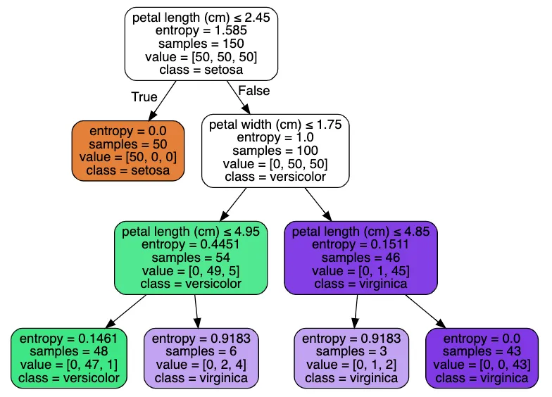 Iris Dataset Decision Tree
Conclusion
Decision trees are powerful tools for both classification and regression tasks. They are easy to interpret and flexible, making them an excellent choice for many machine learning problems. However, care must be taken to prevent overfitting, which can be mitigated by using techniques such as pruning or by using ensemble methods like Random Forests or Gradient Boosting.
By implementing decision trees from scratch, we not only deepen our understanding of the algorithm but also gain the ability to customize it to better suit specific tasks.
Full Code
1
2
3
4
5
6
7
8
9
10
11
12
13
14
15
16
17
18
19
20
21
22
23
24
25
26
27
28
29
30
31
32
33
34
35
36
37
38
39
40
41
42
43
44
45
46
47
48
49
50
51
52
53
54
55
56
57
58
59
60
61
62
63
64
65
66
67
68
69
70
71
72
73
74
75
76
77
78
79
80
81
82
83
84
85
86
87
88
89
90
91
92
93
94
95
96
97
98
99
100
101
102
103
104
105
106
107
108
109
110
111
112
113
114
115
116
117
118
119
120
121
122
123
124
125
126
127
128
129
130
131
132
133
134
135
136
137
138
139
140
141
142
143
144
145
146
147
148
149
150
151
152
153
154
155
156
157
158
159
160
161
162
163
164
165
166
167
168
169
170
171
172
173
174
175
176
177
178
179
180
181
182
183
184
185
import numpy as np

class Node:
    def __init__(self,feature_index=None,threshold=None,condition_mark=None,left=None,right=None,score=None,criterion=None,information_gain=None,label=None):
        self.feature_index = feature_index
        self.threshold = threshold
        self.condition_mark = condition_mark
        self.left = left
        self.right = right
        self.score = score
        self.criterion = criterion
        self.information_gain = information_gain
        self.label = label

class DecisionTree:
    def __init__(self,max_depth=5,min_samples_count=3,criterion='entropy'):
        self.max_depth = max_depth
        self.min_samples_count = min_samples_count
        self.tree = None
        self.criterion = criterion
        self.depth = 0

    def _should_stop(self,data,depth):
        n_labels = len(np.unique(data[:,-1]))
        n_samples = len(data)
        condition = (n_labels == 1) or (n_samples <= self.min_samples_count) or (depth >= self.max_depth)
        return condition

    def _get_label_as_majority(self,data):
        labels,counts = np.unique(data[:,-1],return_counts=True)
        idx_max = np.argmax(counts)
        return labels[idx_max]

    def _get_potential_splits(self,data):
        potential_splits_all = []
        n_features = data.shape[1] - 1 # [feat_1,feat_2,...,feat_n,labels]
        for feature_idx in range(n_features): # iterate over all features
            data_feature = data[:,feature_idx]

            if isinstance(data_feature[0],str) or isinstance(data_feature[0],bool):
                thresholds = np.unique(data_feature)
                condition_mark = '=='
                potential_splits_all.append({'idx':feature_idx,'thresholds':thresholds,'condition_mark':condition_mark})
            else:
                thresholds = [np.median(data_feature)]
                condition_mark = '<='
                potential_splits_all.append({'idx':feature_idx,'thresholds':thresholds,'condition_mark':condition_mark})
        return potential_splits_all

    def _find_best_split(self,data,potential_splits):
        bests = {'feature_index':None,'threshold':None,'condition_mark':None,
                   'information_gain':-float("inf"),'impurity':None,'left_idxs':None,'right_idxs':None}

        labels = data[:,-1]

        for row in potential_splits:
            feature_idx = row["idx"]
            thresholds = row["thresholds"]
            condition_mark = row["condition_mark"]
            features = data[:,feature_idx]

            for threshold in thresholds:
                if condition_mark == '==': # for categorical features
                    cond = np.array([x == threshold for x in features])
                else: # for numerical features
                    cond = np.array([x <= threshold for x in features])

                left_idxs = np.where(cond)[0]
                right_idxs = np.where(~cond)[0]
                information_gain,impurity = self._calculate_information_gain(labels, left_idxs, right_idxs)
                if information_gain > bests['information_gain']:
                    dct = {'feature_index':feature_idx,'threshold':threshold,
                           'condition_mark':condition_mark,'information_gain':information_gain,'impurity':impurity,
                           'left_idxs':left_idxs,'right_idxs':right_idxs}
                    bests.update(dct)

        return bests


    def _calculate_information_gain(self,labels, left_idxs, right_idxs):
        if len(left_idxs) == 0 or len(right_idxs) == 0 :
            information_gain, weighted_impurity = 0 ,0
            return information_gain, weighted_impurity
        else:
            p_left = len(left_idxs) / len(labels)
            p_right = 1 - p_left

            weighted_impurity = p_left * self._calculate_impurity(labels[left_idxs]) + p_right * self._calculate_impurity(labels[right_idxs])
            parent_impurity = self._calculate_impurity(labels)

            information_gain = parent_impurity - weighted_impurity
            return information_gain, weighted_impurity

    def _calculate_impurity(self,labels):
        if self.criterion == 'gini':
            return self._calculate_gini(labels)
        elif self.criterion == 'entropy':
            return self._calculate_entropy(labels)
        else:
            raise Exception("Criterion must be 'gini' or 'entropy'.")

    def _calculate_entropy(self,labels):
        _,counts= np.unique(labels,return_counts=True)
        probs = counts / np.sum(counts)
        score = -np.sum(probs*np.log2(probs+1e-9))# Add small value to avoid log(0)
        return score

    def _calculate_gini(self,labels):
        _,counts= np.unique(labels,return_counts=True)
        probs = counts / np.sum(counts)
        score = 1 - np.sum(np.power(probs,2))
        return score

    def _build_tree(self,data,depth=0):
        if self._should_stop(data,depth):
            leaf_label = self._get_label_as_majority(data)
            return Node(label=leaf_label)
        else:
            potential_splits = self._get_potential_splits(data)
            bests = self._find_best_split(data,potential_splits)

            left_tree = self._build_tree(data = data[bests['left_idxs']],depth=depth+1)
            right_tree = self._build_tree(data = data[bests['right_idxs']],depth = depth+1)

            return Node(feature_index=bests['feature_index'],threshold=bests['threshold'],
                        condition_mark=bests['condition_mark'],left=left_tree,right=right_tree,
                        score=bests['impurity'],criterion=self.criterion,
                        information_gain=bests['information_gain'])

    def fit(self,X,y):
        data = np.column_stack((X,y))
        self.tree = self._build_tree(data)

    def predict(self,X):
        predictions = [self._traverse_tree(data_point, self.tree) for data_point in X]
        return predictions

    # Traverse the tree recursively to predict the label
    def _traverse_tree(self, data_point, node):
        if node.label is not None:  # If we're at a leaf, return the label
            return node.label

        if node.condition_mark == '==':
            if data_point[node.feature_index] == node.threshold:
                return self._traverse_tree(data_point, node.left)
            else:
                return self._traverse_tree(data_point, node.right)
        else:
            if data_point[node.feature_index] <= node.threshold:
                return self._traverse_tree(data_point, node.left)
            else:
                return self._traverse_tree(data_point, node.right)


def test_with_iris_dataset():
    from sklearn.datasets import load_iris
    from sklearn.model_selection import train_test_split
    from sklearn.metrics import accuracy_score

    data = load_iris()
    X, y = data.data, data.target

    # Split the data into training and testing sets
    X_train, X_test, y_train, y_test = train_test_split(X, y, test_size=0.2, random_state=42)

    tree = DecisionTree(max_depth=3, min_samples_count=2, criterion='gini')
    tree.fit(X_train, y_train)

    # Make predictions on the test set
    y_pred = tree.predict(X_test)

    # Calculate accuracy
    accuracy = accuracy_score(y_test, y_pred)
    print(f"Gini Test accuracy: {accuracy * 100:.2f}%")

    # Create and train the decision tree with 'entropy' criterion
    tree_entropy = DecisionTree(max_depth=3, min_samples_count=2, criterion='entropy')
    tree_entropy.fit(X_train, y_train)

    # Make predictions on the test set using entropy criterion
    y_pred_entropy = tree_entropy.predict(X_test)

    # Calculate accuracy
    accuracy_entropy =  accuracy_score(y_test, y_pred_entropy)
    print(f"Entropy Test accuracy: {accuracy_entropy * 100:.2f}%")