Classification Evaluation Metrics in Machine Learning

When building a machine learning model, particularly for classification tasks, one of the most critical aspects is evaluating its performance. You can’t simply rely on a model’s ability to make predictions without knowing how accurate or useful those predictions are. For example, in a healthcare setting, the consequences of misclassifying a patient with a serious illness can be grave, while in an email spam detection system, false positives might just mean a few harmless emails getting flagged as spam. Therefore, understanding classification evaluation metrics is key to developing reliable, effective models that meet specific real-world demands.

Many new data scientists or machine learning engineers jump straight into using metrics like accuracy without fully appreciating its limitations—especially when dealing with imbalanced datasets, where accuracy might give a false sense of model performance. In this blog post, we’ll break down the various classification evaluation metrics, including sensitivity, specificity, true positive rate (TPR), and false positive rate (FPR), alongside precision and recall. We will also explore their mathematical underpinnings and use real-life examples to better illustrate their importance.

The Confusion Matrix: A Foundation for Metrics

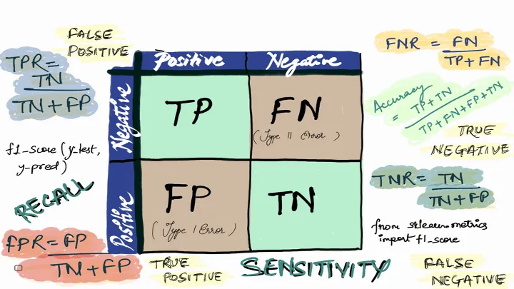
A good place to start is the confusion matrix, which provides a structured way to view the performance of a classification model. It offers a breakdown of how the model’s predictions compare with actual outcomes, and is essential for deriving more nuanced metrics.

The confusion matrix is a table like this:

#	Predicted Positive	Predicted Negative
Actual Positive	True Positive (TP)	False Negative (FN)
Actual Negative	False Positive (FP)	True Negative (TN)

• True Positives (TP): These are the cases where the model correctly predicted the positive class.
• True Negatives (TN): These are instances where the model correctly predicted the negative class.
• False Positives (FP): Here, the model incorrectly predicted the positive class when the actual outcome was negative. Also known as Type I errors.
• False Negatives (FN): These are cases where the model predicted the negative class, but the actual outcome was positive. Known as Type II errors.

With this matrix, we can compute several key metrics to assess model performance from different angles, depending on the problem we’re addressing.

Accuracy: Simple but Misleading

The most straightforward metric derived from the confusion matrix is accuracy.

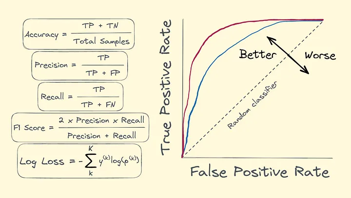
\[\text{Accuracy} = \frac{TP+TN}{FP+FN+TP+TN​}\]

Accuracy measures the proportion of correct predictions out of all predictions. While intuitive and easy to compute, it’s not always reliable, especially in cases of imbalanced datasets. Consider a fraud detection system where only 1% of transactions are fraudulent. A model that predicts “non-fraud” for every transaction would achieve 99% accuracy, but it wouldn’t be effective at actually detecting fraud, which is the goal.

Let’s say we are building a model to classify email as spam or not. We have the following confusion matrix after testing the model on 1000 emails:

#	Predicted Spam	Predicted Not Spam
Actual Spam	30	70
Actual Not Spam	20	880

Here, the accuracy would be:

\[\text{Accuracy} = \frac{TP+TN}{FP+FN+TP+TN​} = \frac{30+880}{30+880+20+70} = \text{0.91}\]

However, this high accuracy hides the fact that the model only catches 30 of the 100 spam emails—thus failing to flag 70 of them.

Precision and Recall: Targeting Specific Error Types

This is where precision and recall come into play. These metrics give you more insight into how the model performs with respect to false positives and false negatives.

Precision

Precision answers the question: “Out of all the positive predictions, how many were correct?”

Precision is particularly important in scenarios where false positives are costly, such as fraud detection or medical diagnoses.

\[\text{Precision} = \frac{TP}{TP+FP}\]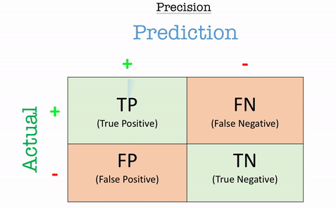

If we calculate precision for email classification example from above:

\[\text{Precision} = \frac{30}{30+20} = 0.60\]

This means that the model only identified 60% of emails flagged as spam were actually spam.

Recall (Sensitivity / True Positive Rate - TPR)

Recall answers the question:“Out of all the actual positives, how many did the model correctly identify?”

Recall, also known as sensitivity or true positive rate (TPR).A high recall means that the model has identified most of the actual positive cases. This is critical in scenarios where missing a positive case (i.e., a false negative) is costly, such as in detecting serious illnesses. For example, In medical testing, recall is key when identifying patients with a disease. If a test has high sensitivity, it correctly identifies a large proportion of those who have the disease, minimizing the chance of missing a sick patient.

\[\text{Recall} = \frac{TP}{TP+FN}\]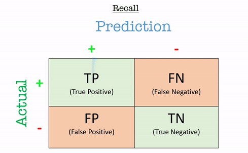

If we calculate recall for email classification example from above:

\[\text{Recall} = \frac{30}{30+70} = 0.30\]

This means that the model only identified 30% of all actual spam emails, leaving 70% of them undetected.

Specificity and False Positive Rate (FPR)

While recall focuses on the true positives, specificity (also known as true negative rate or TNR) and false positive rate (FPR) evaluate the model’s ability to handle the negative class.

Specificity (True Negative Rate - TNR)

Specificity answers the question: “Out of all the actual negatives, how many were correctly identified?”

\[\text{Specificity} = \frac{TN}{TN+FP}\]

High specificity is critical in scenarios where false positives are undesirable, such as in spam detection systems where legitimate emails should not be mistakenly classified as spam.

False Positive Rate (FPR)

The false positive rate (FPR) complements specificity and answers the question: “Out of all the actual negatives, how many were incorrectly predicted as positive?”

\[\text{FPR} = \frac{FP}{FP+TN}\]

In a cancer screening test, specificity helps reduce the number of healthy patients who are falsely flagged for additional, possibly stressful testing. Meanwhile, FPR quantifies how often a healthy individual would be incorrectly classified as needing further screening.

In an ideal model, we want the FPR to be as low as possible, meaning fewer false alarms.

The F1-Score: Balancing Precision and Recall

When precision and recall conflict, the F1-score is a useful metric that balances both. The F1-score is the harmonic mean of precision and recall:

\[\text{F1} = 2 \times \frac {Precision \times Recall}{Precision + Recall}\]

This metric is particularly helpful when dealing with imbalanced datasets and when the cost of false positives and false negatives is similar.

For email example:

\[\text{F1} = 2 \times \frac {0.60 \times 0.30}{0.60 + 0.30}= 2 \times \frac{0.18}{0.90} \approx 0.40\]

The F1-score of 40% shows that neither precision nor recall is exceptionally high, and there’s room for improvement.

AUC-ROC: Understanding the Trade-Offs

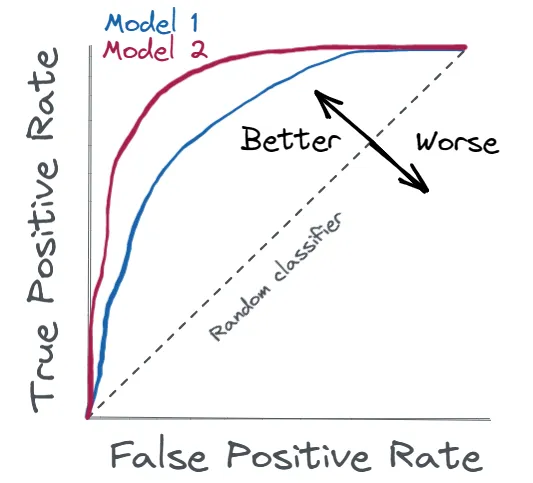AUC-ROC (TPR-FPR Curve)

Another powerful tool for classification evaluation is the ROC curve (Receiver Operating Characteristic) and its corresponding metric, AUC (Area Under the Curve). The ROC curve (Receiver Operating Characteristic) plots the trade-off between the true positive rate (recall) and the false positive rate (FPR) at various thresholds. The AUC-ROC (Area Under the Curve) summarizes this trade-off,An AUC close to 1 indicates excellent model performance, while an AUC around 0.5 suggests the model is no better than random guessing.

\[\text{AUC-ROC} = \text{Area under the ROC Curve} = \int_{0}^{1} \text{TPR}(x) \, d(\text{FPR}(x))\]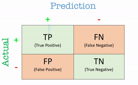

For example, In credit card fraud detection, a high AUC-ROC score indicates that the model does a good job distinguishing between fraudulent and legitimate transactions, even when the dataset is imbalanced.

Precision-Recall Curve

For problems with highly imbalanced classes, the precision-recall curve is often more informative than the ROC curve. It plots precision against recall at different thresholds, helping to find the right balance between catching positive cases and avoiding false positives.

More Real Life Examples

Credit Card Fraud Detection

In this scenario, we are building a classification model to detect fraudulent credit card transactions. Out of 100,000 transactions, only 1,000 are fraudulent, which makes this an imbalanced dataset (fraudulent transactions represent only 1% of the total). We aim to evaluate the performance of a model designed to detect these fraudulent transactions.

Confusion Matrix

	Predicted Fraud (Positive)	Predicted Not Fraud (Negative)
Actual Fraud (Positive)	800	200
Actual Not Fraud (Negative)	9,000	90,000

From this confusion matrix:

• True Positives (TP) = 800 (correctly identified fraudulent transactions)
• False Negatives (FN) = 200 (missed fraudulent transactions)
• False Positives (FP) = 9,000 (incorrectly flagged legitimate transactions as fraud)
• True Negatives (TN) = 90,000 (correctly identified legitimate transactions)
• Accuracy = $\large\frac{800+90000}{800+90000+9000+200} \approx\small 0.908$
• Precision = $\large\frac{800}{800+9000} \approx \small0.081$
• Recall (Sensivity) = $\large\frac{800}{800+200} \approx \small0.80$
• Specificity = $\large\frac{90000}{90000+9000} \approx \small0.909$
• F1 Score = $2\times\large\frac{0.081\times0.80}{0.081 + 0.80} \approx \small0.15$

Even though the Accuracy seems high at 90.8%, it doesn’t tell us much about the model’s ability to detect fraud in an imbalanced dataset. Precision is very low, meaning that out of all the transactions flagged as fraud, only 8.1% were actually fraudulent. This is critical, as we want a model that minimizes false alarms for customers. Recall is high, meaning that the model caught 80% of all fraudulent transactions. This is important in fraud detection, where catching as many fraud cases as possible is crucial. Specificity tells us that 90.9% of the legitimate transactions were correctly classified, which is a good rate for protecting legitimate users. F1-score is 15%, indicating that the balance between precision and recall is not optimal. We might need to tune our model to reduce false positives without sacrificing too much recall.

Illness Detection (Cancer Screening)

Now, let’s consider a cancer screening test for a rare type of cancer that affects 2% of the population. The dataset contains 10,000 patients, with 200 of them actually having the disease. We evaluate the performance of a classification model designed to detect the disease.

Confusion Matrix

	Predicted Positive (Cancer)	Predicted Negative (No Cancer)
Actual Positive (Cancer)	180	20
Actual Negative (No Cancer)	400	9,400

From this confusion matrix:

• True Positives (TP) = 180 (correctly identified cancer cases)
• False Negatives (FN) = 20 (missed cancer cases)
• False Positives (FP) = 400 (healthy patients incorrectly flagged as having cancer)
• True Negatives (TN) = 9,400 (correctly identified healthy patients)
• Accuracy = $\large\frac{180+9400}{180+9400+400+20} \approx \small0.958$
• Precision = $\large\frac{180}{180+400} \approx \small0.31$
• Recall (Sensivity) = $\large\frac{180}{180+20} \approx \small0.90$
• Specificity = $\large\frac{9400}{9400+400} \approx \small0.96$
• F1 Score = $2\times\large\frac{0.31\times0.90}{0.31 + 0.90} \approx \small0.46$

The Accuracy of 95.8% looks great on the surface, but let’s examine the other metrics to get a better understanding. Precision is low at 31%, meaning that many patients who were flagged as having cancer do not actually have the disease. This could lead to unnecessary stress and further testing for those 400 healthy patients.Recall is high, indicating that the model is effective at catching 90% of actual cancer cases. This is crucial in medical screening, as we want to minimize false negatives and ensure most sick patients are detected. A specificity of 96% means that the model correctly identified a high proportion of healthy patients, reducing the risk of false positives. The F1-score is 46%, which balances the low precision with the high recall. While the model is good at identifying cancer cases, its tendency to falsely diagnose healthy patients requires further tuning.

Practical Insights from the Example

In both examples, we see the importance of considering multiple evaluation metrics:

• In fraud detection, recall is critical to catch as many fraud cases as possible, but the low precision indicates too many false alarms, which could frustrate users.
• In cancer screening, high recall is essential to ensure that nearly all patients with cancer are detected, but the low precision means many healthy individuals are incorrectly flagged for further testing, which can cause unnecessary concern.

By evaluating models with precision, recall, specificity, and F1-score, you can choose metrics that best suit your problem. In highly imbalanced datasets, such as fraud detection and illness screening, accuracy alone can be misleading, making these other metrics essential for a clear understanding of model performance.

Comparing the Metrics

The table below summarizes key classification evaluation metrics and their ideal use cases:

Metric	Formula	Best Use Case	Pros	Cons
Accuracy	$\large\frac{TP+TN}{FP+FN+TP+TN​}$ ​	Balanced datasets	Easy to compute	Misleading in imbalanced datasets
Precision	$\large\frac{TP}{TP+FP}$	When false positives are costly	Minimizes false positives	Ignores false negatives
Recall (Sensitivity / TPR)	$\large\frac{TP}{TP+FN}$	​ When false negatives are costly	Catches more true positives	Can lead to more false positives
Specificity (TNR)	$\large\frac{TN}{TN+FP}$	​ When true negatives are important	Minimizes false positives	Ignores false negatives
F1-Score	$\large\text{2 x }\frac{Precision \times Recall}{Precision + Recall}$	When balance between precision and recall is needed	Balances precision and recall	Harder to interpret than individual metrics
AUC-ROC	$\text{Area Under the ROC Curve}$	Imbalanced datasets with binary classification	Provides insight into model discrimination ability	Less useful for highly skewed datasets
FPR	​ $\large\frac{FP}{FP+TN}$	When reducing false alarms is crucial	Helps assess false alarms	Can be high in imbalanced datasets

Conclusion

In conclusion, the selection of metrics depends on the nature of the problem and the trade-offs between different types of errors. While accuracy is easy to understand, it often falls short in real-world applications, especially with imbalanced datasets. Metrics such as precision, recall, sensitivity, and specificity provide a more nuanced view of the model’s performance. By carefully selecting the most appropriate metrics, you can develop models that are not only performant in theory but also suited to real-world demands.